7  Report 1

Linear and logistic regression

The goal of this report is to review and consolidate what we learned together in the first block of the course. You are not required to do anything that we have not already seen.

For students enrolled in this course in the Winter Semester 2023/24: The report is due January 11, 2024 at 11:59pm, but I encourage you to submit before the holidays if you have the capacity to do so. Please submit your Quarto script, as well as a rendered copy (preferably HTML, but PDF is also fine) to Moodle (under ‘Reports’).

7.1 Dataset

For this report you will continue using the data from Biondo et al. (2022), an eye-tracking reading study on adverb-tense congruence effects on reading time measures. Participants’ eye movements were recorded as they read Spanish sentences where temporal adverbs and verb tense were either congruent or incongruent. For both sentence regions, the time reference was either past (e.g., yesterda, bought) or future (e.g., tomorrow, will buy). Example stimuli from this experiment are given in Table 14.1. You will be fitting models to different eye-tracking reading measures from this experiment, with the predictors verb tense and grammaticality.

Table 7.1: Example stimuli

sentence	adverb	verb	gramm
A la salida del trabajo, **ayer** las chicas **compraron** pan en la tienda.<br> *After leaving work* **yesterday** *the girls* **bought** *bread at the shop*	past	past	gramm
A la salida del trabajo, **ayer** las chicas **\*comprarán** pan en la tienda.<br> *After leaving work* **yesterday** *the girls* **\*will buy** *bread at the shop*	past	future	ungramm
A la salida del trabajo, **mañana** las chicas **comprarán** pan en la tienda.<br> *After leaving work* **tomorrow** *the girls* **will buy** *bread at the shop*	future	future	gramm
A la salida del trabajo, **mañana** las chicas **\*compraron** pan en la tienda.<br> *After leaving work* **tomorrow** *the girls* **\*bought** *bread at the shop*	future	past	ungramm

7.2 Set-up

Make sure you begin with a clear working environment. To achieve this, you can go to Session > Restart R. Your Environment should have no objects in it, and you should not have any packages loaded.

7.2.1 Packages

Load the packages below. Give a short description of why we load in each package, i.e., what these packages help us do (1-2 sentences each). Tip: remember you can type ?tidyverse into the Console to get an overview of a package or function.

pacman::p_load(
  tidyverse,
  janitor,
  here,
  broom
)

1. tidyverse:
2. janitor:
3. here:

7.2.2 Data

Run the code below. Give a short description of what each line of code does (you can skip the locale line). Tip: roi == 2 corresponds to the temporal adverb condiiton.

df_tense <-
  read_csv(here("data", "Biondo.Soilemezidi.Mancini_dataset_ET.csv"),
           locale = locale(encoding = "Latin1") ## for special characters in Spanish
           ) |> 
  clean_names() |> 
  mutate(gramm = ifelse(gramm == "0", "ungramm", "gramm"))  |> 
  filter(roi == 2,
         adv_type == "Deic") |> 
  mutate(length = nchar(label))

You can write your answer like this, for example:

1. df_tense <- :
2. read_csv:
3. clean_names:
4. mutate:
5. filter:

7.3 How to report your models

You will be running linear and logisitc regression models. Our variables of interest will be:

variable	description	type	class
`fp`	first-pass reading time (summation of fixations from when a reader first fixates on a region to when they first leave that region)	dependent	continuous
`tt`	total reading time (summation of all fixations within a region during a trial)	dependent	continuous
`ri`	regressions in (whether there was at least one regression into a region)	dependent	binomial
`ro`	regressions out (whether there was at least one regression out of a region)	dependent	binomial
`verb_t`	verb tense: past or future	independent	categorical
`gramm`	grammaticality: grammatical or ungrammatical	independent	categorical
`length`	region length in letters	independent	continuous

7.3.1 Example model report

Imagine we fit a linear model, called fit_verb_tt, to log-tranformed total reading times at the verb region. Our fixed effects (i.e., predictors) are verb tense, grammaticality, and their interaction. Below I report the findings of the model, which is what you should aim to do with the models you run.

The model summary is given in ?tbl-fit_verb_tt, with back-transformed model predictions visualised in Figure 7.1. A main effect of grammaticality was found in total reading times at the verb region, with ungrammatical conditions eliciting longer total reading times than grammatical conditions (Est = -0.06, t = -2.4, p < 0.05). A main effect of tense was also found, with the future condition eliciting longer total reading times than the past condition (Est = 0.07, t = 2.48, p < .05). An interaction of tense and grammaticality was not significant (Est = 0.04, t = 1).

library(papaja)

fit_verb_tt |> 
  apa_print() |>
  apa_table(label = "tbl-fit_verb_tt",
            caption = "Model summary for (log-transformed) total reading times at the verb region.")

(#tab:unnamed-chunk-12) Model summary for (log-transformed) total reading times at the verb region.

Predictor	\(b\)	95% CI	\(t\)	\(\mathit{df}\)	\(p\)
Intercept	6.22	[6.19, 6.26]	332.72	3791	< .001
Verb tPast	-0.06	[-0.11, -0.01]	-2.38	3791	.017
Grammungramm	0.07	[0.01, 0.12]	2.47	3791	.013
Verb tPast \(\times\) Grammungramm	0.04	[-0.04, 0.11]	1.01	3791	.312

library(sjPlot)
plot_model(fit_verb_tt, type = "int") + 
  geom_line(position = position_dodge(0.1)) +
  labs(title = "Predicted total reading times at the verb region",
       x = "Verb tense",
       y = "Reading time (ms)") +
  theme_bw()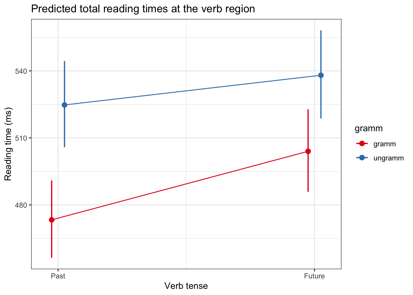

Figure 7.1: Back-transformed model predictions for total reading time at the verb region (with 95% confidence intervals).

7.4 Variable prep

We need to prepare our predictors: centering continuous variables and sum contrast coding categorical variables.

7.4.1 Centring continuous variables

Create a new variable length_c which contains the centred values of length (just centre, you don’t need to standardise). Centre using the median rather than the mean (hint: there is a function median()).

7.4.2 Contrast coding

Set sum contrast coding for tense and gramm. You might need to first use the as.factor() function to save the variables as factors. Your contrasts should look like this:

contrasts(df_tense$gramm)

        [,1]
gramm   -0.5
ungramm  0.5

contrasts(df_tense$verb_t)

       [,1]
Future  0.5
Past   -0.5

7.5 Linear regression

We run linear regression when we have a continuous dependent variable. You will be fitting a. model to first-pass reading time.

7.5.1 Fitting our model

Fit a model of log-transformed first-pass reading times with verb tense, grammaticality, and their interaction as fixed effects (hint: you might want to use * in your model).

7.5.2 Assessing assumptions

Visually assess the model assumptions of normality and homoscedasticity and write 1-2 sentences about each assumption, referring to the figures you produced.

7.5.3 Extracting predictions

1. Create objects intercept, b1 (verb_t), and b2 (gramm) that contain the corresponding model coefficient estimate for each term (hint: each object should contain a single value, which corresponds to the estimate for this term in your model summary output).

2. Generate the fitted values for each of our four conditions. We covered a number of ways to do this in class:

   1. Using our model formula (\(\ref{eq-fp}\)) and the sum contrast values for each level of verb_t and gramm (i.e., +/-0.5, given in Table 7.2), compute the back-transformed predicted total reading time for each condition. Recall: \(b_0\) is our intercept, \(b_1\) is our slope for verb_t (i.e., the value of the object you just named verb_t), and \(b_2\) is our slope (estimate) for gramm (i.e., the value of the object you just named gramm).
   2. The ggeffects package: we used the ggeffect() function, but the ggpredict() function back-transforms the estimates for us.

\[\begin{equation} fp = exp(b_0 + b_1*verb\_t + b_2*gramm) \label{eq-fp} \end{equation}\]

Table 7.2: Corresponding value of factor levels to be plugged into equation ef{eq-fp}

	-0.5	+0.5
`verb_t`	past	future
`gramm`	gramm	ungramm

7.5.4 Report model

Write a short report of the model findings. Produce a table and plot like in the example above to supplement your report.

7.6 Logistic regression

We run logistic regression when we have a binimial dependent variable. You will be fitting a logistic regression model to regression in.

7.6.1 Fit model

Fit a generalied linear model (logistic regression) to the regression in data, with the same fixed effects as your linear model above (verb_t, gramm, and their interaction). Remember, you will need a different function (not lm), and to add another argument (family = ...).

7.6.2 Interpretation

Write a short report of the model findings. Produce a table and plot like in the example above to supplement yor report. Recall that our coefficient estimates are in log odds).

Biondo, N., Soilemezidi, M., & Mancini, S. (2022). Yesterday is history, tomorrow is a mystery: An eye-tracking investigation of the processing of past and future time reference during sentence reading. Journal of Experimental Psychology: Learning, Memory, and Cognition, 48(7), 1001–1018. https://doi.org/10.1037/xlm0001053