4  Multiple Regression

Regression for Linguists

Author

Affiliation

Daniela Palleschi

Humboldt-Universität zu Berlin

Summary

• we saw that the equation for a straight line boils down to its intercept and slope
• we fit our first linear model with a continuous predictor

Learning Objectives

Today we will learn…

• what multiple regression is
• how to include multiple predictor variables
• how to interpret slopes in multiple regression
• how to interpret interaction effects
• about the assumption of the absence of collinearity

Set-up environment

# suppress scientific notation
options(scipen=999)

We’ll also need to load in our required packages. Hopefully you’ve already install the required packages (if not, go to Chapter 3).

# load libraries
pacman::p_load(
               tidyverse,
               here,
               broom,
               janitor,
               languageR)

Load data

We’ll use the full dataset of the frequency data.

df_freq_full <-
  read_csv(here("data", "ELP_full_length_frequency.csv")) |> 
  clean_names() |> 
  mutate(freq = 10^(log10freq), # inverse log10
         freq_log = log(freq)) |>  # use natural logarithm
  relocate(word, rt, length, freq, freq_log)

We have 4 variables:

• word
• length
• rt
• freq
• freq_log
• log10freq

4.1 Multiple regression

So far we’ve worked with simple linear models, which fit a model to a predictor and response variable. These models do not differ so greatly from a one- or two-sample t-test (for a categorical predictor) or Pearson’s r (for a standardised continuous predictor). You might be wondering then we would bother with linear regression. One reason is that it allows us to include multiple predictors in our models, which still boils down to modeling the mean, but while condintioning the mean on multiple variables at once.

Recall the equation of a line (\(\ref{eq-simple-lin-2}\)), which states that any value of \(y\) equals the intercept (\(b_0\)) plus the corresponding value of \(x\) multiplied by the slope (\(b_1x\)), plus the error, which are our residuals (\(e\)). In multiple regression, we can include more than one slope (\(\ref{eq-multiple-reg}\)).

\[\begin{align} y &= b_0 + b_1x + e \label{eq-simple-lin-2} \\ y &= b_0 + b_1x + b_2x + ... + e \label{eq-multiple-reg} \end{align}\]

flowchart LR
  A[Continuous variable] 
  A --> F[Zero-truncated with positive skew \n e.g., reaction times]
  A --> H[Interval i.e., lower and upperbound \n e.g., rating scale]
  H --> I[Centre on median value]
  I --> E(Response)
  E --> Z[Done]
  F --> G[Non-linear transformation \n e.g., log-transform]
  G --> B(Predictor)
  I --> B(Predictor)
  B --> C{One predictor}
  C --> X[Centre]
  D --> Y[Centre and standardise]
  B --> D{Two predictor}
  G --> E(Response)
  
  

Figure 4.1: Flowchart of common steps for linear and non-linear transformations of continuous variables. Such decision trees are not a one-size-fits-all solution and cannot replace critical thinking and understanding of your data.

4.1.1 One predictor

Let’s re-run our simple model with this dataset. Let’s keep reaction times in the raw milliseconds for now for interpretability.

fit_freq_full <-
  lm(rt ~ log(freq), data = df_freq_full)

tidy(fit_freq_full)

# A tibble: 2 × 5
  term        estimate std.error statistic p.value
  <chr>          <dbl>     <dbl>     <dbl>   <dbl>
1 (Intercept)    907.      1.09       828.       0
2 log(freq)      -37.5     0.262     -143.       0

We see there is a decrease in reaction times (-37.5 milliseconds) for a 1-unit increase in log frequency. Let’s look at the model fit using glance().

glance(fit_freq_full)$r.squared

[1] 0.3834186

We see that the R-squared is 0.383, meaning our model describes 38% of the variance in response times. We can’t be sure that this described variance is due solely to frequency, however. Our models only know what we tell them! Other effects that are correlated with frequency might be conflating the frequency effect, e.g., more frequent words tend to be shorter (zipf_1949?). Let’s expand our model to include word length [\(\ref{eq-freq-length}\)].

\[\begin{equation} y = b_0 + b_1*log frequency + b_2*word length \label{eq-freq-length} \end{equation}\]

4.1.2 Adding a predictor

Let’s add length as a predictor to our model.

fit_freq_mult <-
  lm(rt ~ log(freq) + length, data = df_freq_full)

tidy(fit_freq_mult) |> select(term, estimate)

# A tibble: 3 × 2
  term        estimate
  <chr>          <dbl>
1 (Intercept)    748. 
2 log(freq)      -29.5
3 length          19.5

We see that length is also a significant predictor of reaction times, with an increase in word length (+1 letter) corresponds to a 20ms increase in reaction times. Our intercept is also now 748ms, instead of 907ms. The 907ms intercept corresponds to the prediction for reaction times to a word with 0 log frequency and 0 word length, but this is not very interpretable. If we were to center both prdictors, the intercept would be the reaction time for a wrd with average frequency and average length.

The slope for log frequency has also changed: from -37.5 to -29.5. This change tells us that some of the effect in our first model was confounded with length, as controlling for length weakens the effect of frequency.

glance(fit_freq_mult)$r.squared

[1] 0.4872977

We also see that including length increases the variance described by our model, reflected in the R-squared values (0.4872977 instead of 0.3834186.

4.2 Standardising our predictors

Recall that, when we have multiple continuous predictors, standardising them can help their interpretation, as their slopes are comparable. We could achieve this by centering each variable and then dividing by the standard deviation, or we could use the scale() function, which does just this.

# centre and then standardize
df_freq_full |> 
  mutate(
         freq_z1 = (freq-mean(freq))/sd(freq),
         freq_z2 = scale(freq)) |> 
  select(freq_z1, freq_z2) |> 
  head()

# A tibble: 6 × 2
  freq_z1 freq_z2[,1]
    <dbl>       <dbl>
1 -0.0902     -0.0902
2 -0.0864     -0.0864
3 -0.0905     -0.0905
4 -0.0864     -0.0864
5 -0.0885     -0.0885
6 -0.0901     -0.0901

Let’s use scale() for freq and length.

df_freq_full <-
  df_freq_full |> 
  mutate(freq_z = scale(freq_log),
         length_z = scale(length))

fit_freq_z <-
  lm(rt ~ freq_z + length_z, data = df_freq_full)

First, let’s check the \(R^2\):

glance(fit_freq_z)$r.squared

[1] 0.4872977

We see that our \(R^2\) value is 0.4872977, just like above. This serves as a reminder that the predictors still represent the same variance in the underlying model, their units and scales have simply changed. What about our coefficients:

tidy(fit_freq_z) |> select(term, estimate)

# A tibble: 3 × 2
  term        estimate
  <chr>          <dbl>
1 (Intercept)    770. 
2 freq_z         -60.6
3 length_z        43.3

Here, a 1-unit change always corresponds to a change of 1 standard deviation. Now we see that frequency has a larger magnitude than the effect of length. So, for each instease in frequency by 1 standard deviation (holiding length constant), reaction times decrease by 29.5 ms.

4.2.1 Adding an interaction term

We won’t spent much time talking about interactions, but please check out Ch. 8 (Interations and nonlinear effects) in Winter (2019) for a more in-depth treatment. For now, what’s important to know is that interactions describe how effects of one predictor may be influenced by changes in another predictor. We can add interactin terms of two predictors by connecting them with a colon (:).

lm(rt ~ freq_z + length_z + freq_z:length_z, 
   data = df_freq_full) |> 
  tidy() |> select(term, estimate)

# A tibble: 4 × 2
  term            estimate
  <chr>              <dbl>
1 (Intercept)        766. 
2 freq_z             -63.9
3 length_z            41.8
4 freq_z:length_z    -11.4

Or, we can simply connect the two predictors with an asterisk (*) to indicate that we want to look at both predictors and their interaction.

lm(rt ~ freq_z*length_z, 
   data = df_freq_full) |> 
  tidy() |> select(term, estimate)

# A tibble: 4 × 2
  term            estimate
  <chr>              <dbl>
1 (Intercept)        766. 
2 freq_z             -63.9
3 length_z            41.8
4 freq_z:length_z    -11.4

The model estimates are the same for both models. The intercept is the predicted reaction time for a word with the mean length and mean frequency. Notice that the interaction slope is negative, meaning when both freq and length increase, reaction times will decrease.

4.3 Model assumptions

We’ve already discussed the assumptions of normality and homoscedasticity (constant variance), which both refer to the residuals of a model. We typically assess these assumptions visually, with histogram and Q-Q plots.

4.3.1 Normality and Homoscedasticity

For our model

fig_hist <-
fit_freq_z |> 
  ggplot() +
  aes(x = .resid) +
  geom_histogram(bins = 20, fill = "grey", colour = "black") +
  theme_bw() +
  labs(title='Histogram', x='Residuals', y='Count')

fig_qq <-
fit_freq_z |> 
  ggplot() +
  aes(sample = .resid) +
  geom_qq(colour = "red") +
  geom_qq_line() +
  labs(title='Q-Q Plot', x='Theoretical quantiles', y='Sample quantiles')

fig_res <-
  fit_freq_z |> 
  ggplot() +
  aes(x = .fitted, y = .resid) +
  geom_point() +
  geom_hline(yintercept = 0, colour = "blue") +
  labs(title='Residual vs. Fitted Values Plot', x='Fitted Values', y='Residuals')

fig_hist + fig_qq + fig_res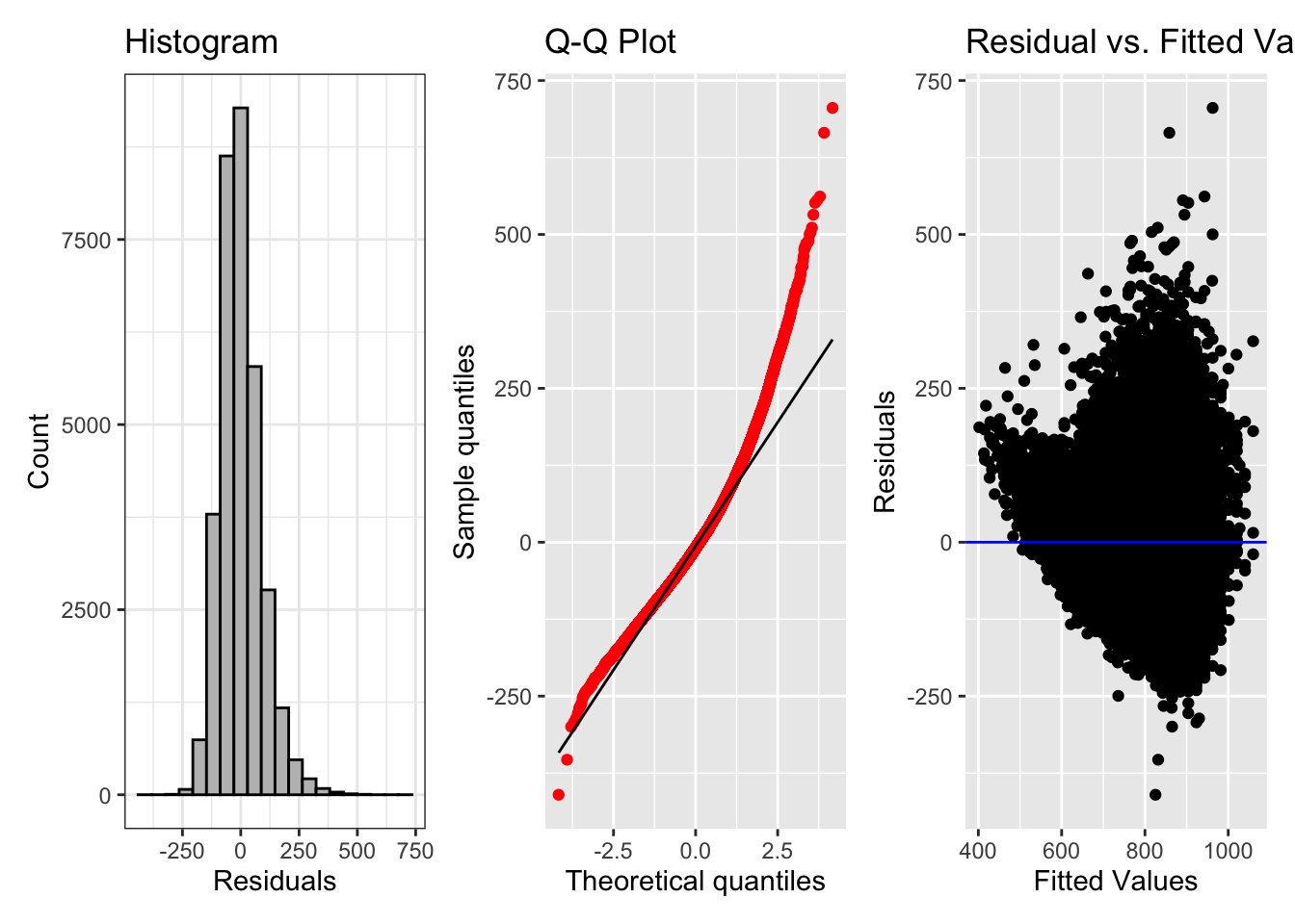

The histogram looks approximately normally distributed, with a bit of a positive skew. The Q-Q plot suggests a less-normal distribution, with the model estimates fitting larger reaction times more poorly. The residual plot also shows that the variance of the residuals is not constant, with much larger residual variance for larger fitted values. This tells us we should probably log reaction times. Let’s try it all again, with log-transformed reaction times.

4.3.2 Log-transformed response variable

fit_freq_log_z <-
  lm(log(rt) ~ freq_z*length_z,
     data = df_freq_full)

glance(fit_freq_log_z)$r.squared

[1] 0.5176913

tidy(fit_freq_log_z) |> select(term, estimate)

# A tibble: 4 × 2
  term            estimate
  <chr>              <dbl>
1 (Intercept)      6.63   
2 freq_z          -0.0826 
3 length_z         0.0524 
4 freq_z:length_z -0.00779

We see now that our values are much smaller, because they’re on the log-scale.

exp(6.63 + -0.0826*5 + 0.0524*2)

[1] 556.5739

exp(6.63 + -0.0826*4 + 0.0524*2)

[1] 604.499

exp(6.63 + -0.0826*1 + 0.0524*6)

[1] 955.0847

tidy(fit_freq_log_z)

# A tibble: 4 × 5
  term            estimate std.error statistic  p.value
  <chr>              <dbl>     <dbl>     <dbl>    <dbl>
1 (Intercept)      6.63     0.000636   10428.  0       
2 freq_z          -0.0826   0.000666    -124.  0       
3 length_z         0.0524   0.000649      80.7 0       
4 freq_z:length_z -0.00779  0.000581     -13.4 8.51e-41

fig_hist <-
fit_freq_log_z |> 
  ggplot() +
  aes(x = .resid) +
  geom_histogram(bins = 20, fill = "grey", colour = "black") +
  theme_bw() +
  labs(title='Histogram', x='Residuals', y='Count')

fig_qq <-
fit_freq_log_z |> 
  ggplot() +
  aes(sample = .resid) +
  geom_qq(colour = "red") +
  geom_qq_line() +
  labs(title='Q-Q Plot', x='Theoretical quantiles', y='Sample quantiles')

fig_res <-
  fit_freq_log_z |> 
  ggplot() +
  aes(x = .fitted, y = .resid) +
  geom_point() +
  geom_hline(yintercept = 0, colour = "blue") +
  labs(title='Residual vs. Fitted Values Plot', x='Fitted Values', y='Residuals')

fig_hist + fig_qq + fig_res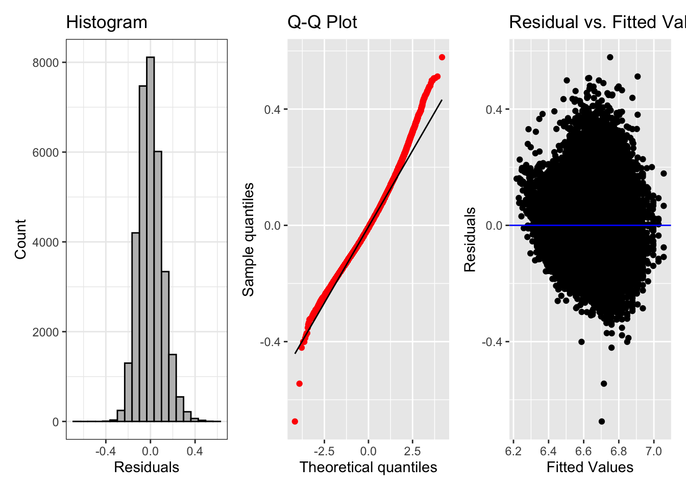

Looks much better.

4.3.3 Collinearity

Collinearity refers to when continuous predictor variables are correlated, which can make the interpretation of their coefficients difficult, and the results spurious. Regression assumes there is an absence of collinearity, i.e., our predictor variables are not correlatded.

To assess collinearity, you can use the vif() function from the car package to compare variance inflation factors. VIF values close to 1 indicates there is not a high degree of collinearity between your variables.

car::vif(fit_freq_log_z)

         freq_z        length_z freq_z:length_z 
       1.246509        1.184641        1.068283 

Collinearity is a conceptual problem, and is something that you need to consider in the planning stage. Typically, we want to include predictors that we have specific predictions or research questions about. Shoving a bunch of predictors in a model to see what comes out significant is bad practice. Rather, we should have a principled approach to model building and variable selection. This is not to say that exploratory analyses should be avoided, but that this comes with caveats.

4.3.4 Adjusted \(R^2\)

Although we should avoid throwing any old predictor into our model, adjusted \(R^2\) is a more conservative version of \(R^2\) that takes into account the number of predictors in a model. For each additional predictor, adjusted \(R^2\) includes the number of predictors (\(k\)) in its denominator (bottom half of a division), which means that the more predictors there are, the smaller \(R^2\) will be, unless each additional predictor explains sufficient variance to counteract this penalisation.

glance(fit_freq_log_z)$adj.r.squared

[1] 0.5176475

If we were to look at the (adjusted) \(R^2\) of our simple linear regression model, where log reaction times are predicted by standardised log frequency, we see that there is a large increase in our model which includes length and its interaction. This suggests that our model is not overfit, and that length contributes to the variance explained by the model.

glance(lm(log(rt) ~ freq_z, data = df_freq_full))$adj.r.squared

[1] 0.4148675

If we likewise compare to the same model without an interaction term (log reaction times ~ frequency * length), we see that the adjusted \(R^2\) is not very different. If the adjusted \(R^2\) were much lower, this would indicate that including the interaction term leads to overfitting.

glance(lm(log(rt) ~ freq_z + length_z, data = df_freq_full))$adj.r.squared

[1] 0.5150461

Important terms

Term	Definition	Equation/Code
Collinearity	Correlation between two predictors (linear model assumes non-collinearity)	car::vif(model)

Learning Objectives 🏁

Today we learned…

• what multiple regression is
• how to include multiple predictor variables
• how to interpret slopes in multiple regression
• how to interpret interaction effects
• about the assumption of the absence of collinearity

4.4 Task

Load in the english dataset from the languageR package (Baayen & Shafaei-Bajestan, 2019) (code below). You don’t need to load in any CSV file, because this dataset is available if you have the package loaded. From the manual:

This data set gives mean visual lexical decision latencies and word naming latencies to 2284 monomorphemic English nouns and verbs, averaged for old and young subjects, with various predictor variables.

(languageR manual, p. 29)

# load in 'english' dataset from languageR
df_freq_eng <-
  as.data.frame(english) |> 
  dplyr::select(RTlexdec, RTnaming, Word, LengthInLetters, AgeSubject, WrittenFrequency) |> 
  rename(rt_lexdec = RTlexdec,
         rt_naming = RTnaming,
         freq_written = WrittenFrequency) |> 
  clean_names() |> 
  relocate(word)

We’re keeping five variables:

• word: a factor with 2284 words
• rt_lexdec: numeric vector of log RT in visual lexical decision
• rt_naming: numeric vector of log RT in word naming
• length_in_letters: numeric vector with length of the word in letters
• AgeSubject: a factor with as levels the age group of the subject: young versus old.
• freq_written: numeric vector with log frequency in the CELEX lexical database

Take the following steps:

1. Perform an exploratory data analysis to understand the data (produce plots, tables, whatever you think necessary and can do).

2. Model the data, with back-transformed (raw) reaction times as a response variable and written frequency and length in letters as predictors. Perform any tranformations you think necessary. Run model diagnostic checks and assess model fit.

3. Re-run the model with log reaction times as a response variable and written frequency and length in letters as predictors. Perform any tranformations you think necessary. Run model diagnostic checks and assess model fit.

4. Remove length in letters as a predictor. How is model fit affected? What can you conclude?

Session Info

Developed with Quarto using R version 4.4.0 (2024-04-24) (Puppy Cup) and RStudio version 2023.9.0.463 (Desert Sunflower), and the following packages:

sessionInfo()

R version 4.4.0 (2024-04-24)
Platform: aarch64-apple-darwin20
Running under: macOS Ventura 13.2.1

Matrix products: default
BLAS:   /Library/Frameworks/R.framework/Versions/4.4-arm64/Resources/lib/libRblas.0.dylib 
LAPACK: /Library/Frameworks/R.framework/Versions/4.4-arm64/Resources/lib/libRlapack.dylib;  LAPACK version 3.12.0

locale:
[1] en_US.UTF-8/en_US.UTF-8/en_US.UTF-8/C/en_US.UTF-8/en_US.UTF-8

time zone: Europe/Berlin
tzcode source: internal

attached base packages:
[1] stats     graphics  grDevices datasets  utils     methods   base     

other attached packages:
 [1] googlesheets4_1.1.1 gt_0.10.1           kableExtra_1.4.0   
 [4] knitr_1.43          patchwork_1.2.0     languageR_1.5.0    
 [7] janitor_2.2.0       broom_1.0.5         here_1.0.1         
[10] lubridate_1.9.3     forcats_1.0.0       stringr_1.5.1      
[13] dplyr_1.1.4         purrr_1.0.2         readr_2.1.5        
[16] tidyr_1.3.1         tibble_3.2.1        ggplot2_3.5.1      
[19] tidyverse_2.0.0    

loaded via a namespace (and not attached):
 [1] gtable_0.3.5      xfun_0.40         htmlwidgets_1.6.4 gargle_1.5.2     
 [5] tzdb_0.4.0        vctrs_0.6.5       tools_4.4.0       generics_0.1.3   
 [9] curl_5.2.1        parallel_4.4.0    fansi_1.0.6       pacman_0.5.1     
[13] pkgconfig_2.0.3   lifecycle_1.0.4   farver_2.1.1      compiler_4.4.0   
[17] munsell_0.5.1     carData_3.0-5     snakecase_0.11.1  sass_0.4.7       
[21] htmltools_0.5.8.1 yaml_2.3.7        car_3.1-2         crayon_1.5.2     
[25] pillar_1.9.0      abind_1.4-5       tidyselect_1.2.1  digest_0.6.33    
[29] stringi_1.8.3     labeling_0.4.3    rprojroot_2.0.4   fastmap_1.1.1    
[33] grid_4.4.0        colorspace_2.1-0  cli_3.6.2         magrittr_2.0.3   
[37] utf8_1.2.4        withr_3.0.0       scales_1.3.0      backports_1.4.1  
[41] bit64_4.0.5       googledrive_2.1.1 timechange_0.3.0  httr_1.4.7       
[45] rmarkdown_2.24    bit_4.0.5         cellranger_1.1.0  hms_1.1.3        
[49] evaluate_0.21     viridisLite_0.4.2 rlang_1.1.3       glue_1.7.0       
[53] xml2_1.3.6        renv_1.0.7        svglite_2.1.3     rstudioapi_0.16.0
[57] vroom_1.6.5       jsonlite_1.8.7    R6_2.5.1          systemfonts_1.0.6
[61] fs_1.6.3         

References

Baayen, R. H., & Shafaei-Bajestan, E. (2019). languageR: Analyzing linguistic data: A practical introduction to statistics. https://CRAN.R-project.org/package=languageR

Winter, B. (2019). Statistics for Linguists: An Introduction Using R. In Statistics for Linguists: An Introduction Using R. Routledge. https://doi.org/10.4324/9781315165547