13  Model selection: Example

Parsimonious model selection

Author

Affiliation

Daniela Palleschi

Humboldt-Universität zu Berlin

Under construction

This chapter is not fully translated from bullet points (from my slides) to prose. This will happen eventually (hopefully by spring 2024).

Learning Objectives

Today we will…

• apply remedies for nonconvergence
• reduce our RES with a data-driven approach
• compare a parsimonious model to maximal and intercept-only models

Resources

• this lecture covers
  • Sections 10.3-5 in Sonderegger (2023)
  • Section 15.7.3 ‘Convergence Issues’ in Winter (2019)
  • Brauer & Curtin (2018)
  • Meteyard & Davies (2020)
• we will continue using the data from Biondo et al. (2022)

Set-up

# suppress scientific notation
options(scipen=999)

Code for a function to format p-values

library(broman)
# function to format p-values
format_pval <- function(pval){
    dplyr::case_when(
        pval < .001 ~ "< .001",
        pval < .01 ~ "< .01",
        pval < .05 ~ "< .05",
        TRUE ~ broman::myround(pval, 3)
    )
}

Load packages

# load libraries
pacman::p_load(
               tidyverse,
               here,
               janitor,
               # new packages for mixed models:
               lme4,
               lmerTest,
               broom.mixed,
               lattice)

lmer <- lmerTest::lmer

Load data

• data from Biondo et al. (2022)

df_biondo <-
  read_csv(here("data", "Biondo.Soilemezidi.Mancini_dataset_ET.csv"),
           locale = locale(encoding = "Latin1") ## for special characters in Spanish
           ) |> 
  clean_names() |> 
  mutate(gramm = ifelse(gramm == "0", "ungramm", "gramm")) |> 
  mutate_if(is.character,as_factor) |> # all character variables as factors
  droplevels() |> 
  filter(adv_type == "Deic")

13.0.1 Set contrasts

contrasts(df_biondo$verb_t) <- c(-0.5,+0.5)
contrasts(df_biondo$gramm) <- c(-0.5,+0.5)

contrasts(df_biondo$verb_t)

       [,1]
Past   -0.5
Future  0.5

contrasts(df_biondo$gramm)

        [,1]
gramm   -0.5
ungramm  0.5

13.1 Start maximal

• model structure should be decided a priori
  • included fixed (predictors and covariates) and random effects

13.1.1 Maximal model

• starting point: most maximal model structure justified by your design
  • if this converges, great!
  • if it doesn’t, what does this mean and what should we do?

fit_verb_fp_mm <- lmer(log(fp) ~ verb_t*gramm + 
                      (1 + verb_t*gramm|sj) +
                      (1 + verb_t*gramm|item),
                    data = df_biondo,
                    subset = roi == 4)

• we get a warning of singular fit

13.2 Convergence issues

• “Convergence is not a metric of model quality” (Sonderegger, 2023, p. 365, Box 10.2)
  • convergence does not always indicate “overfitting” or “overparameterisation”
  • can also be due to optimizer choice
    • since default optimizer was changed to nloptwrap from bobyqa, there seem to be more ‘false positive’ convergence warnings
• false-positive convergence: you get a convergence warning, but changing the optimizer and/or iteration count does not produce a warning
• false-negative convergence: you do not get a warning, but your variance-covariance matrix might indicate overfitting

13.2.1 Nonconvergence remedies

• unfortunately there is no one “right” way to deal with convergence issues
  • important is to transparently report and justify your method
• Table 17 in Brauer & Curtin (2018) (p. 404) suggests 20 remedies, whittled down to 10 suggestions in Sonderegger (2023)

Figure 13.1: From Sonderegger (2023), p. 366

13.2.2 Intrusive vs. Non-intrusive remedies

• non-intrusive remedies amount to checking/adjusting data and model specifications

• intrusive remedies involve reducing random effects structure

  • there are different schools of thought
    • random-intercepts only: increased Type I error rate = overconfident estimates
    • maximal-but-singular-fit model (Barr et al., 2013): reduces power = underconfident estimates
    • data-driven approach (Bates et al., 2015): can lose the forest for the trees, e.g., removing random slopes for predictors of interest

• each strategy has its drawback

  • important is to choose your strategy a priori and transparently report and justify your strategy
  • even better: share/publish your data and code, which should be reproducible

13.2.3 ?convergence

• type ?convergence in the Console and read the vignette
  • what suggestions does it make?
• compare this to ?isSingular

13.3 Non-intrusive methods

• check your data structure/variables
  • check model assumptions (e.g., normality, missing transformations of variables)
  • check your RES is justified by your experimental design/data structure
  • centre your predictors (e.g., sum contrasts, or centring/standardizing) to reduce multicollinearity; reduces collinearity in the random effects (a possible source of nonconvergence)
  • check observations per cell (e.g., is there a participant very few observations, or few observations per one condition? Should be at least >5 per cell)
• alter model controls:
  • increase iterations
  • check optimizer

13.3.1 Check optimzer

• optimizer
  • lme4::allFit(model) (can take a while to run)

all_fit_verb_fp_mm <- allFit(fit_verb_fp_mm)
# bobyqa : boundary (singular) fit: see help('isSingular')
# [OK]
# Nelder_Mead : [OK]
# nlminbwrap : boundary (singular) fit: see help('isSingular')
# [OK]
# nmkbw : [OK]
# optimx.L-BFGS-B : boundary (singular) fit: see help('isSingular')
# [OK]
# nloptwrap.NLOPT_LN_NELDERMEAD : boundary (singular) fit: see help('isSingular')
# [OK]
# nloptwrap.NLOPT_LN_BOBYQA : boundary (singular) fit: see help('isSingular')
# [OK]
# There were 11 warnings (use warnings() to see them)

13.3.2 Optimizers

• default optimizer for lmer() is nloptwrap, formerly bobyqa (Bound Optimization by Quaradric Approximiation)

  • usually changing to bobyqa helps

• see ?lmerControl for more info

• if fits are very similar (or all optimizeres except the default), the nonconvergent fit was a false positive

  • it’s safe to use the new optimizer

summary(all_fit_verb_fp_mm)$llik

                       bobyqa                   Nelder_Mead 
                    -2105.109                     -2179.479 
                   nlminbwrap                         nmkbw 
                    -2105.106                     -2105.109 
              optimx.L-BFGS-B nloptwrap.NLOPT_LN_NELDERMEAD 
                    -2105.106                     -2105.106 
    nloptwrap.NLOPT_LN_BOBYQA 
                    -2105.106 

summary(all_fit_verb_fp_mm)$fixef

                              (Intercept)    verb_t1      gramm1 verb_t1:gramm1
bobyqa                           5.956403 0.06170602 0.003369634    -0.01418865
Nelder_Mead                      5.956350 0.06188102 0.003488675    -0.01397531
nlminbwrap                       5.956403 0.06170726 0.003369637    -0.01419047
nmkbw                            5.956404 0.06170653 0.003369153    -0.01419036
optimx.L-BFGS-B                  5.956403 0.06170717 0.003369787    -0.01419044
nloptwrap.NLOPT_LN_NELDERMEAD    5.956403 0.06170725 0.003369649    -0.01419046
nloptwrap.NLOPT_LN_BOBYQA        5.956403 0.06170771 0.003369203    -0.01419184

13.3.3 Increase iterations

• and/or increase number of iterations
  • default is 10 000 (1e5 in scientific notation)
  • you can try 20 000, 100 000, etc.
  • this usually helps with larger data or models with complex RES

# check n of iterations
fit_verb_fp_mm@optinfo$feval

[1] 2318

13.3.4 lmerControl()

fit_verb_fp_mm <- lmer(log(fp) ~ verb_t*gramm + 
                      (1 + verb_t*gramm|sj) +
                      (1 + verb_t*gramm|item),
                    data = df_biondo,
                    subset = roi == 4,
                    control = lmerControl(optimizer = "bobyqa",
                                          optCtrl = list(maxfun = 2e5))
)

• or you can just ‘update’ the model to save some syntax

fit_verb_fp_mm <- update(fit_verb_fp_mm,
                         control = lmerControl(optimizer = "bobyqa", 
                                                optCtrl = list(maxfun = 2e5)))

boundary (singular) fit: see help('isSingular')

Warning: Model failed to converge with 1 negative eigenvalue: -5.3e-01

13.3.5 Removing parameters

• still won’t converge?
  • it’s time to consider intrusive remedies: removing random effects parameters

13.4 Intrusive methods

• nonconvergence in maximal models is often due to overfitting
  • i.e., the model is overly complex given your data
  • this is typically due to an overly complex random effects structure
• if the non-intrusive methods don’t lead to convergence, the problem is likely overfitting

13.4.1 Parsimonious vs. maximal

• there are different camps on how to deal with this issue
• I personally follow the suggestions in Bates et al. (2015) (for now)
  1. run random effects Principal Components Analysis (summary(rePCA(model)), lme4 package)
     • informs by how many parameters our model is overfit
  2. check variance-covariance matrix (VarCorr(model))
  3. remove parameters with very high or low Correlation terms and/or much lower variance compared to other terms
  4. fit simplified model
  5. wash, rinse, repeat
• we’ll practice this method today, but keep in mind that it’s up to you to decide and justify which method you use

13.4.2 Random effects Principal Components Analysis

• gives us a ranking of all parameters (‘components’) in our RES per unit

summary(rePCA(fit_verb_fp_mm))

$item
Importance of components:
                         [,1]   [,2]    [,3]                    [,4]
Standard deviation     0.3638 0.2493 0.08366 0.000000000000000001309
Proportion of Variance 0.6567 0.3085 0.03474 0.000000000000000000000
Cumulative Proportion  0.6567 0.9653 1.00000 1.000000000000000000000

$sj
Importance of components:
                         [,1]    [,2]        [,3]          [,4]
Standard deviation     0.6490 0.01470 0.000001281 0.00000001467
Proportion of Variance 0.9995 0.00051 0.000000000 0.00000000000
Cumulative Proportion  0.9995 1.00000 1.000000000 1.00000000000

13.4.2.1

• important is the Cumulative Proportion
  • how much of the cumulative variance explained by all the by-unit parameters does this one parameter contribute?
  • we see for item, the first component accounts for 66% of the variance explained, and the next contributes an additional 31%, and the next 3%
  • so two components account for roughly 97% of variance explained by our RES
  • in other words, we can remove one component for sure, and possibly another
  • we could potentially remove 3 components from participant

13.4.3 Variance-covariance matrix

• so we can remove 2 parameters from item and participant
  • so either the varying intercept, or slope for tense, grammaticality, or their interaction
• we can check this with VarCorr(fit_verb_fp_mm)

VarCorr(fit_verb_fp_mm)

 Groups   Name           Std.Dev. Corr                
 item     (Intercept)    0.139189                     
          verb_t1        0.055890  0.488              
          gramm1         0.022569 -0.109 -0.921       
          verb_t1:gramm1 0.095314 -0.283  0.456 -0.646
 sj       (Intercept)    0.257535                     
          verb_t1        0.018296 0.974               
          gramm1         0.012055 0.960  0.872        
          verb_t1:gramm1 0.017731 0.991  0.934  0.990 
 Residual                0.399095                     

• for item I would remove gramm because it has the lowest variance, and has a pretty high correlation with verb_t (which is unlikely to be true)
• I would also remove gramm for participant for the same reason, as well as its high correlation with the intercept and verb_t

13.4.3.1 Alternate model 1

• for now let’s just remove the interaction term
  • for reproducibility reasons, do not delete the code for a model that did not converge
  • rather, write a comment on what decision was made (and why) for the new model

fit_verb_fp_m1 <- lmer(log(fp) ~ verb_t*gramm + 
                      (1 + verb_t+gramm|sj) +
                      (1 + verb_t+gramm|item),
                    data = df_biondo,
                    subset = roi == 4,
                    control = lmerControl(optimizer = "bobyqa",
                                          optCtrl = list(maxfun = 2e5))
)

boundary (singular) fit: see help('isSingular')

13.4.3.1.1 rePCA()

summary(rePCA(fit_verb_fp_m1))

$item
Importance of components:
                         [,1]   [,2]          [,3]
Standard deviation     0.3559 0.1291 0.00000007181
Proportion of Variance 0.8837 0.1163 0.00000000000
Cumulative Proportion  0.8837 1.0000 1.00000000000

$sj
Importance of components:
                         [,1]         [,2] [,3]
Standard deviation     0.6465 0.0000006824    0
Proportion of Variance 1.0000 0.0000000000    0
Cumulative Proportion  1.0000 1.0000000000    1

13.4.3.1.2 VarCorr()

VarCorr(fit_verb_fp_m1)

 Groups   Name        Std.Dev. Corr         
 item     (Intercept) 0.139274              
          verb_t1     0.055550  0.489       
          gramm1      0.020747 -0.117 -0.924
 sj       (Intercept) 0.257657              
          verb_t1     0.017584 1.000        
          gramm1      0.011554 1.000  1.000 
 Residual             0.399869              

• when we see Corr +/-1, this tells us there was an error computing correlations between parameters
  • it is an invitation to explore
• this is not plausible, and indicates overfitting in our model
  • we can remove all slopes from sj

13.4.3.1.3 by-item random effects

lattice::dotplot(ranef(fit_verb_fp_m1))$item

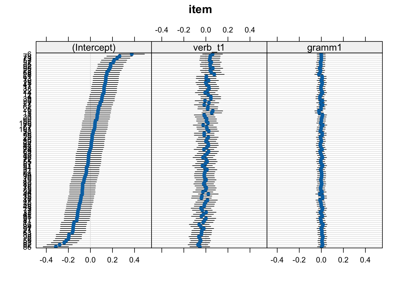
13.4.3.1.4 by-participant random effects (with +1 correlations)

lattice::dotplot(ranef(fit_verb_fp_m1))$sj

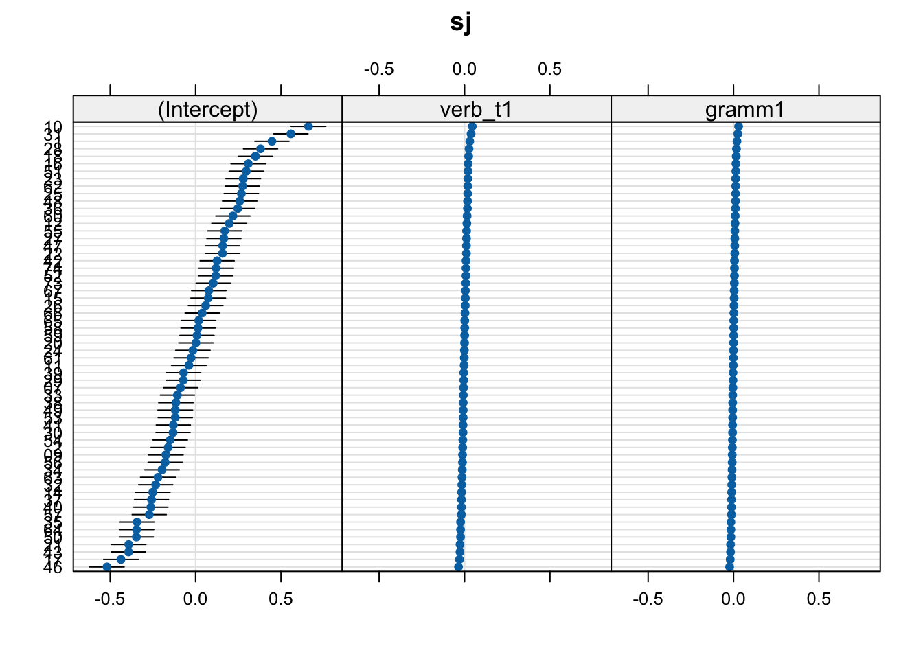
13.4.3.2 Alternate model 2

fit_verb_fp_m2 <- lmer(log(fp) ~ verb_t*gramm + 
                      (1 |sj) +
                      (1 + verb_t+gramm|item),
                    data = df_biondo,
                    subset = roi == 4,
                    control = lmerControl(optimizer = "bobyqa",
                                          optCtrl = list(maxfun = 2e5))
)

boundary (singular) fit: see help('isSingular')

13.4.3.2.1 rePCA()

summary(rePCA(fit_verb_fp_m2))

$item
Importance of components:
                         [,1]   [,2]          [,3]
Standard deviation     0.3559 0.1297 0.00000001647
Proportion of Variance 0.8827 0.1173 0.00000000000
Cumulative Proportion  0.8827 1.0000 1.00000000000

$sj
Importance of components:
                         [,1]
Standard deviation     0.6441
Proportion of Variance 1.0000
Cumulative Proportion  1.0000

13.4.3.2.2 VarCorr()

VarCorr(fit_verb_fp_m2)

 Groups   Name        Std.Dev. Corr         
 item     (Intercept) 0.139364              
          verb_t1     0.055805  0.485       
          gramm1      0.020546 -0.097 -0.917
 sj       (Intercept) 0.257648              
 Residual             0.399995              

• by-item slopes for gramm and verb_t are highly correlated
• gramm has least variance, so let’s remove it

13.4.3.2.3 by-item random effects

lattice::dotplot(ranef(fit_verb_fp_m2))$item

13.4.3.3 Alternate model 3

fit_verb_fp_m3 <- lmer(log(fp) ~ verb_t*gramm + 
                      (1 |sj) +
                      (1 + verb_t|item),
                    data = df_biondo,
                    subset = roi == 4,
                    control = lmerControl(optimizer = "bobyqa",
                                          optCtrl = list(maxfun = 2e5))
)

• converged!

13.4.3.3.1 rePCA()

summary(rePCA(fit_verb_fp_m3))

$item
Importance of components:
                         [,1]    [,2]
Standard deviation     0.3553 0.10311
Proportion of Variance 0.9223 0.07768
Cumulative Proportion  0.9223 1.00000

$sj
Importance of components:
                         [,1]
Standard deviation     0.6438
Proportion of Variance 1.0000
Cumulative Proportion  1.0000

13.4.3.3.2 VarCorr()

VarCorr(fit_verb_fp_m3)

 Groups   Name        Std.Dev. Corr 
 item     (Intercept) 0.139365      
          verb_t1     0.050134 0.542
 sj       (Intercept) 0.257714      
 Residual             0.400315      

13.4.3.4 Alternate model 4

• but we might’ve also decided to remove verb_t, so let’s run that model

fit_verb_fp_m4 <- lmer(log(fp) ~ verb_t*gramm + 
                      (1 |sj) +
                      (1 + gramm|item),
                    data = df_biondo,
                    subset = roi == 4,
                    control = lmerControl(optimizer = "bobyqa",
                                          optCtrl = list(maxfun = 2e5))
)

boundary (singular) fit: see help('isSingular')

• does not converge, so we’re justified in keeping by-item verb_t slopes

13.4.4 Final model

• the final model name should be some sort of convention to make your life easier
  • so remove model index

fit_verb_fp <- fit_verb_fp_m3

13.4.4.0.1 by-item random effects

lattice::dotplot(ranef(fit_verb_fp))$sj

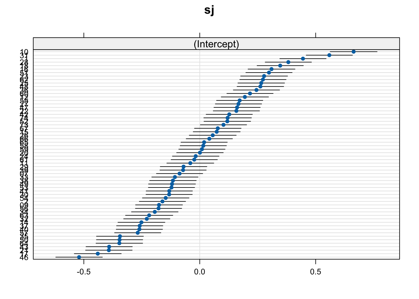
13.4.4.0.2 by-participant random effects

lattice::dotplot(ranef(fit_verb_fp))$item

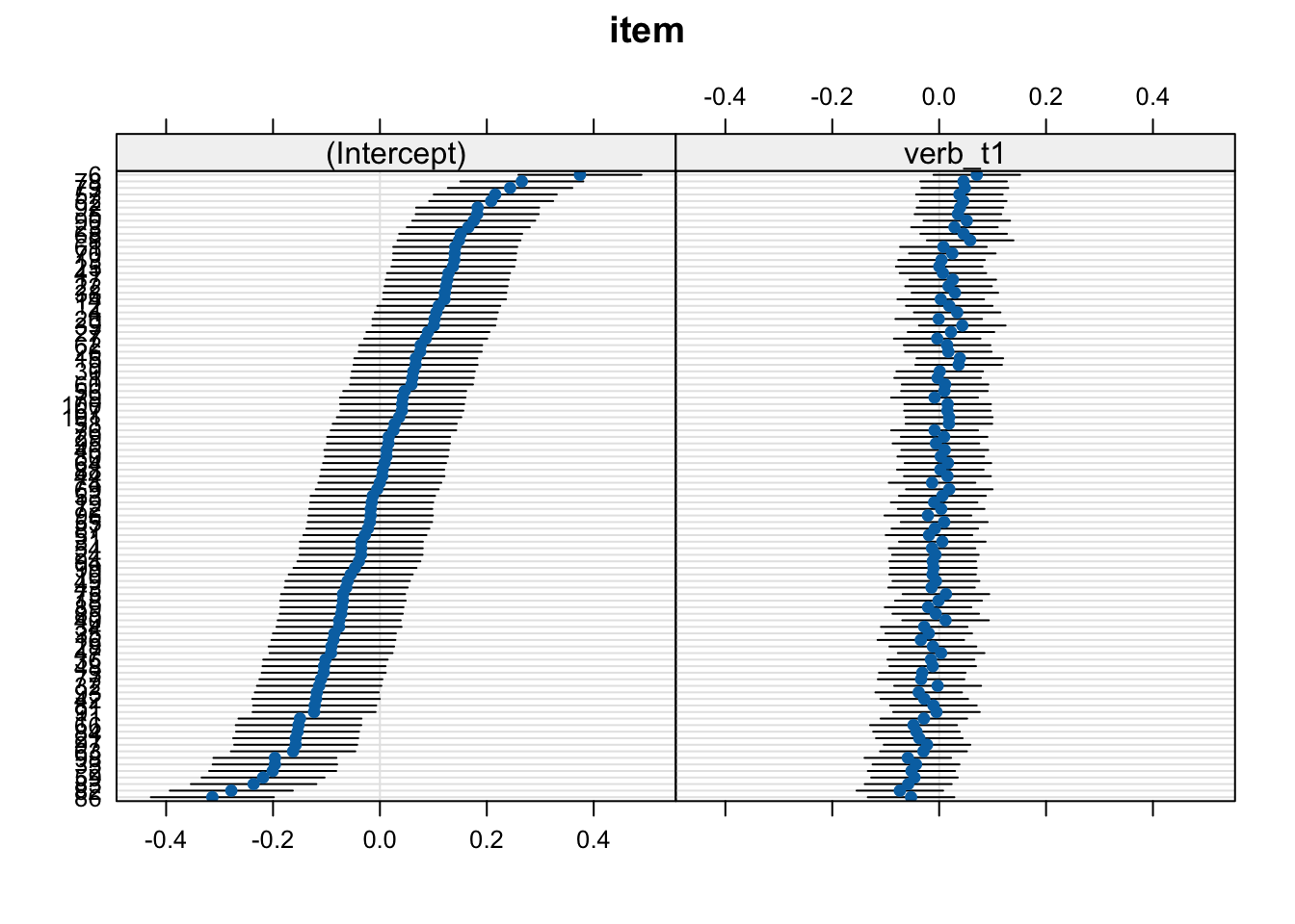
13.4.4.0.3 summary()

summary(fit_verb_fp)

Linear mixed model fit by REML. t-tests use Satterthwaite's method [
lmerModLmerTest]
Formula: log(fp) ~ verb_t * gramm + (1 | sj) + (1 + verb_t | item)
   Data: df_biondo
Control: lmerControl(optimizer = "bobyqa", optCtrl = list(maxfun = 200000))
 Subset: roi == 4

REML criterion at convergence: 4216.2

Scaled residuals: 
    Min      1Q  Median      3Q     Max 
-4.1758 -0.6096 -0.0227  0.6060  4.0568 

Random effects:
 Groups   Name        Variance Std.Dev. Corr
 item     (Intercept) 0.019423 0.13936      
          verb_t1     0.002513 0.05013  0.54
 sj       (Intercept) 0.066417 0.25771      
 Residual             0.160252 0.40032      
Number of obs: 3795, groups:  item, 96; sj, 60

Fixed effects:
                  Estimate  Std. Error          df t value             Pr(>|t|)
(Intercept)       5.956384    0.036763   79.243172 162.021 < 0.0000000000000002
verb_t1           0.061733    0.013971   93.410519   4.419            0.0000267
gramm1            0.003298    0.012999 3544.451690   0.254                 0.80
verb_t1:gramm1   -0.014380    0.025998 3544.762213  -0.553                 0.58
                  
(Intercept)    ***
verb_t1        ***
gramm1            
verb_t1:gramm1    
---
Signif. codes:  0 '***' 0.001 '**' 0.01 '*' 0.05 '.' 0.1 ' ' 1

Correlation of Fixed Effects:
            (Intr) vrb_t1 gramm1
verb_t1      0.077              
gramm1       0.000 -0.002       
vrb_t1:grm1  0.000  0.002  0.000

• IMPORTANTLY, only look at the fixed effects after you’ve got your final model!!!!
  • i.e., run model -> convergence error -> rePCA() + VarCorr() -> run model -> … -> converges -> only NOW run summary(model)

13.5 Comparing to ‘bad’ models

• let’s compare our final model to our ‘bad’ models
  • random intercepts-only model (overconfident)
  • maximal model (underconfident)

13.5.1 Random-intercepts only

fit_verb_fp_intercepts <- lmer(log(fp) ~ verb_t*gramm + 
                      (1 |sj) +
                      (1 |item),
                    data = df_biondo,
                    subset = roi == 4
)

• converges

Code

sum_fit_verb_fp <-
  tidy(fit_verb_fp,
     effects = "fixed") |> 
  as_tibble() |> 
  mutate(p_value = format_pval(p.value),
         model = "parsimonious") 

sum_fit_verb_fp_mm <-
  tidy(fit_verb_fp_mm,
     effects = "fixed") |> 
  as_tibble() |> 
  mutate(p_value = format_pval(p.value),
         model = "maximal") 

sum_fit_verb_fp_intercepts <-
  tidy(fit_verb_fp_intercepts,
     effects = "fixed") |> 
  as_tibble() |> 
  mutate(p_value = format_pval(p.value),
         model = "intercepts")

13.5.2 coefficient estimates

Code

rbind(sum_fit_verb_fp, sum_fit_verb_fp_intercepts, sum_fit_verb_fp_mm) |> 
  select(term, estimate, model) |>
  mutate(estimate = round(estimate,4)) |> 
  pivot_wider(
    id_cols = c(term),
    names_from = model,
    values_from = estimate
  ) |> 
  mutate(measure = "estimate") |> 
  kable() |> 
  kable_styling()

Table 13.1: Coefficient estimates for our parsimonious model, a random-intercepts only model, and a maximal model

term	parsimonious	intercepts	maximal	measure
(Intercept)	5.9564	5.9564	5.9564	estimate
verb_t1	0.0617	0.0619	0.0617	estimate
gramm1	0.0033	0.0032	0.0034	estimate
verb_t1:gramm1	-0.0144	-0.0143	-0.0142	estimate

13.5.3 standard error

Code

rbind(sum_fit_verb_fp, sum_fit_verb_fp_intercepts, sum_fit_verb_fp_mm) |> 
  select(term, std.error, model) |>
  mutate(std.error = round(std.error,4)) |> 
  pivot_wider(
    id_cols = c(term),
    names_from = model,
    values_from = std.error
  ) |> 
  mutate(measure = "std.error") |> 
  kable() |> 
  kable_styling()

Table 13.2: Standard error of coefficient estimates for our parsimonious model, a random-intercepts only model, and a maximal model

term	parsimonious	intercepts	maximal	measure
(Intercept)	0.0368	0.0368	0.0367	std.error
verb_t1	0.0140	0.0130	0.0144	std.error
gramm1	0.0130	0.0130	0.0133	std.error
verb_t1:gramm1	0.0260	0.0260	0.0278	std.error

• standard error (\\(SE = \frac{\sigma}{\sqrt{n}}\\\)) is a measure of uncertainty
  • larger values reflect greater uncertainty
  • because \(n\) is in the denominator, SE gets smaller with more observations
• compared to our parsimonious model with by-item varying verb_t slopes:
  • smaller SE for our overconfident (intercepts) model
  • larger SE for our underconfident (maximal) model
  • but only for the estimate also included in the random effects

13.5.4 t-values

Code

rbind(sum_fit_verb_fp, sum_fit_verb_fp_intercepts, sum_fit_verb_fp_mm) |> 
  select(term, statistic, model) |>
  mutate(statistic = round(statistic,4)) |> 
  pivot_wider(
    id_cols = c(term),
    names_from = model,
    values_from = statistic
  ) |> 
  mutate(measure = "statistic") |> 
  kable() |> 
  kable_styling()

Table 13.3: t-values of each estimates for our parsimonious model, a random-intercepts only model, and a maximal model

term	parsimonious	intercepts	maximal	measure
(Intercept)	162.0213	161.9025	162.1605	statistic
verb_t1	4.4188	4.7517	4.2982	statistic
gramm1	0.2537	0.2466	0.2542	statistic
verb_t1:gramm1	-0.5531	-0.5496	-0.5108	statistic

• t-value (\\(t = \frac{\bar{x}_1 - \bar{x}_2}{SE}\\\)) is a measure of uncertainty
  • larger values reflect greater effect
  • more \(n\) increases \(t\)
• again, verb_t: \(t_{max}\) < \(t_{pars}\) < \(t_{int}\)

13.5.5 degrees of freedom

Code

rbind(sum_fit_verb_fp, sum_fit_verb_fp_intercepts, sum_fit_verb_fp_mm) |> 
  select(term, df, model) |>
  mutate(df = round(df,4)) |> 
  pivot_wider(
    id_cols = c(term),
    names_from = model,
    values_from = df
  ) |> 
  mutate(measure = "df") |> 
  kable() |> 
  kable_styling()

Table 13.4: Degrees of freedom of each estimates for our parsimonious model, a random-intercepts only model, and a maximal model

term	parsimonious	intercepts	maximal	measure
(Intercept)	79.2432	79.2008	79.1789	df
verb_t1	93.4105	3637.1332	71.4491	df
gramm1	3544.4517	3637.1834	179.9254	df
verb_t1:gramm1	3544.7622	3637.1023	91.8597	df

• degrees of freedom: not trivially defined in mixed models; we’re using Satterthwaite approximiation (default in lmerTest::lmer())
  • larger degrees of freedom corresponds to larger \(n\)
  • including more random effects reduces our \(n\) and therefore reduces \(df\)
• again, verb_t: \(df_{max}\) < \(df_{pars}\) < \(df_{int}\)
  • and large differences between our maximal model and the other two for other terms

13.5.6 p-values

Code

rbind(sum_fit_verb_fp, sum_fit_verb_fp_intercepts, sum_fit_verb_fp_mm) |> 
  select(term, p.value, model) |>
  mutate(p.value = round(p.value, 8)) |> 
  pivot_wider(
    id_cols = c(term),
    names_from = model,
    values_from = p.value
  ) |> 
  mutate(measure = "p.value") |> 
  kable() |> 
  kable_styling()

Table 13.5: p-values of coefficient estimates for our parsimonious model, a random-intercepts only model, and a maximal model

term	parsimonious	intercepts	maximal	measure
(Intercept)	0.0000000	0.0000000	0.0000000	p.value
verb_t1	0.0000267	0.0000021	0.0000535	p.value
gramm1	0.7997645	0.8052568	0.7996181	p.value
verb_t1:gramm1	0.5802114	0.5826522	0.6107496	p.value

• p-values: inversely related to t-values (larger t-values = smaller p-values)
• again, verb_t: \(p_{max}\) < \(p_{pars}\) < \(p_{int}\)
  • this would be important for ‘signicance’ if the values were closer to the convential alpha-levels (p < .05, p < .01, p < .001)
  • but here the different random effects structures don’t qualitatively change (all are < .001)
• this is not always the case, however!
  • this is why we do not peek at the fixed effects until we have our final model
  • we don’t want to be influenced (consciously or not) by seeing small p-values in one model but not another

13.6 Reporting

• in Data Analysis section, e.g.,

We included Time Reference (past, future), and Verb Match (match, mismatch) as fixed-effect factors in the models used to investigate the processing of past–future violations (Q1), by adopting sum contrast coding (Schad et al., 2020): past and match conditions were coded as –.5. while future and mismatch conditions were coded as .5. […] Moreover, we included crossed random intercepts and random slopes for all fixed-effect parameters for subject and item grouping factors (Barr et al., 2013) in all models.

We reduced the complexity of the random effect structure of the maximal model by performing a principal component analysis so as to identify the most parsimonious model properly supported by the data (Bates et al., 2015). […] all reading time data were log transformed before performing the analyses.

— Biondo et al. (2022), p. 9

13.6.1 Formatted p-values

• we can use the format_pval() function defined earlier to produce formatted p-values

  tidy(fit_verb_fp,
     effects = "fixed") |> 
  as_tibble() |> 
  mutate(p_value = format_pval(p.value)) |> 
  select(-p.value) |> 
  kable() |> 
  kable_styling()

Table 13.6: Table with formatted p-values from format_pval()

effect	term	estimate	std.error	statistic	df	p_value
fixed	(Intercept)	5.9563839	0.0367630	162.0213327	79.24317	< .001
fixed	verb_t1	0.0617330	0.0139706	4.4187865	93.41052	< .001
fixed	gramm1	0.0032976	0.0129994	0.2536709	3544.45169	0.800
fixed	verb_t1:gramm1	-0.0143804	0.0259984	-0.5531269	3544.76221	0.580

Learning objectives 🏁

Today we…

• applied remedies for nonconvergence ✅
• reduced our RES with a data-driven approach ✅
• compared a parsimonious model to maximal and intercept-only models ✅

Important terms

Term	Definition	Equation/Code
linear mixed (effects) model	NA	NA

References

Barr, D. J., Levy, R., Scheepers, C., & Tily, H. J. (2013). Random effects structure for confirmatory hypothesis testing: Keep it maximal. Journal of Memory and Language, 68(3), 255–278. https://doi.org/10.1016/j.jml.2012.11.001

Bates, D., Kliegl, R., Vasishth, S., & Baayen, H. (2015). Parsimonious Mixed Models. arXiv Preprint, 1–27. https://doi.org/10.48550/arXiv.1506.04967

Biondo, N., Soilemezidi, M., & Mancini, S. (2022). Yesterday is history, tomorrow is a mystery: An eye-tracking investigation of the processing of past and future time reference during sentence reading. Journal of Experimental Psychology: Learning, Memory, and Cognition, 48(7), 1001–1018. https://doi.org/10.1037/xlm0001053

Brauer, M., & Curtin, J. J. (2018). Linear mixed-effects models and the analysis of nonindependent data: A unified framework to analyze categorical and continuous independent variables that vary within-subjects and/or within-items. Psychological Methods, 23(3), 389–411. https://doi.org/10.1037/met0000159

Meteyard, L., & Davies, R. A. I. (2020). Best practice guidance for linear mixed-effects models in psychological science. Journal of Memory and Language, 112, 104092. https://doi.org/10.1016/j.jml.2020.104092

Sonderegger, M. (2023). Regression Modeling for Linguistic Data.

Winter, B. (2019). Statistics for Linguists: An Introduction Using R. In Statistics for Linguists: An Introduction Using R. Routledge. https://doi.org/10.4324/9781315165547