11 Shrinkage and Partial Pooling

Shrinkage of random Complete, No, Partial Pooling

Author

Affiliation

Daniela Palleschi

Humboldt-Universität zu Berlin

Published

January 12, 2024

Modified

February 13, 2024

Under construction

This chapter is not fully translated from bullet points (from my slides) to prose. This will happen eventually (hopefully by spring 2024).

This chapter presents figures from the blog post “Plotting partial pooling in mixed-effects models” from Tristin Mahr (2017). You can also read Section 15.9 'Shrinkage and Individual Differences’ in Winter (2019) and Box 8.2 'Broader Context: Shrinkage and Partial Pooling’ in Sonderegger (2023) for a short overview of the topics of shrinkage and partial pooling. We will be using the data from Biondo et al. (2022).

Learning Objectives

Today we will learn…

about no/complete/partial pooling
about shrinkage

Set-up

# suppress scientific notation
options(scipen=999)

Load packages

# load libraries
pacman::p_load(
               tidyverse,
               janitor,
               here,
               lmerTest)

lmer <- lmerTest::lmer

Load data

data from Biondo et al. (2022)

df_biondo <-
  read_csv(here("data", "Biondo.Soilemezidi.Mancini_dataset_ET.csv"),
           locale = locale(encoding = "Latin1") ## for special characters in Spanish
           ) |> 
  clean_names() |> 
  mutate(gramm = ifelse(gramm == "0", "ungramm", "gramm")) |> 
  mutate_if(is.character,as_factor) |> # all character variables as factors
  droplevels() |> 
  filter(adv_type == "Deic")

11.1 Set contrasts

contrasts(df_biondo$verb_t) <- c(-0.5,+0.5)
contrasts(df_biondo$gramm) <- c(-0.5,+0.5)
contrasts(df_biondo$adv_type) <- c(-0.5,+0.5)

contrasts(df_biondo$verb_t)

       [,1]
Past   -0.5
Future  0.5

contrasts(df_biondo$gramm)

        [,1]
gramm   -0.5
ungramm  0.5

contrasts(df_biondo$adv_type)

         [,1]
Deic     -0.5
Non-deic  0.5

11.2 Run models

random-intercepts only

fit_fp_1 <-
  lmer(log(fp) ~ verb_t*gramm + 
         (1 |sj) +
         (1|item), 
       data = df_biondo, 
       subset = roi == 4)

by-item varying tense slopes

fit_fp_item <-
  lmerTest::lmer(log(fp) ~ verb_t*gramm + 
         (1 |sj) +
         (1 + verb_t|item), 
       data = df_biondo, 
       subset = roi == 4)

12 Pooling

do the random effects represent the exact average of participants?
- below we see the mean logged first-pass reading time per participant (mean) and the by-participant intercepts from fit_fp_1 and fit_fp_item
to understand what’s happening, we first have to understand pooling

Code

sum_shrinkage <- df_biondo |> 
  filter(roi == 4) |> 
  summarise(mean = mean(log(fp), na.rm = T),
            .by = "sj") |> 
  mutate(population_mean = mean(mean, na.rm = T)) |> 
  left_join(coef(fit_fp_1)$sj["(Intercept)"] |> rownames_to_column(var = "sj")) |> 
  rename(intercept_1 = `(Intercept)`) |> 
  left_join(coef(fit_fp_item)$sj["(Intercept)"] |> rownames_to_column(var = "sj")) |> 
  rename(intercept_item = `(Intercept)`) 

sum_shrinkage |> 
  head()

# A tibble: 6 × 5
  sj     mean population_mean intercept_1 intercept_item
  <chr> <dbl>           <dbl>       <dbl>          <dbl>
1 1      6.42            5.96        6.40           6.40
2 2      5.79            5.96        5.79           5.80
3 07     5.87            5.96        5.87           5.87
4 09     5.78            5.96        5.78           5.78
5 10     6.67            5.96        6.62           6.62
6 11     5.91            5.96        5.91           5.92

12.1 No pooling

no pooling refers to separate regression lines fit e.g., per participant
- each regression line is fit ignoring the population-level information
- the intercepts are the true mean from each participant

head(df_no_pooling)

       model sj intercept    verb_t1      gramm1 verb_t1:gramm1
1 No pooling  1  6.422811 0.16094962  0.07844247     0.12950513
2 No pooling  2  5.792669 0.10115512 -0.10571656    -0.23199316
3 No pooling 07  5.870556 0.15344172 -0.25264603    -0.29866189
4 No pooling 09  5.780839 0.16938275  0.14074977    -0.07324559
5 No pooling 10  6.664530 0.04786447 -0.13824470     0.21824110
6 No pooling 11  5.912309 0.07573670 -0.06469794     0.35318406

sum_shrinkage |> head(6)

# A tibble: 6 × 5
  sj     mean population_mean intercept_1 intercept_item
  <chr> <dbl>           <dbl>       <dbl>          <dbl>
1 1      6.42            5.96        6.40           6.40
2 2      5.79            5.96        5.79           5.80
3 07     5.87            5.96        5.87           5.87
4 09     5.78            5.96        5.78           5.78
5 10     6.67            5.96        6.62           6.62
6 11     5.91            5.96        5.91           5.92

12.2 Complete pooling

complete pooling refers to ignoring grouping factors
- i.e., fixed-effects only models (e.g., with lm() or glm())
- one regression line fit ignoring the individual-level information
- the intercepts are the same as the population-level mean

head(df_pooled)

# A tibble: 6 × 6
  model            sj    intercept verb_t1  gramm1 `verb_t1:gramm1`
  <chr>            <fct>     <dbl>   <dbl>   <dbl>            <dbl>
1 Complete pooling 1          5.96  0.0612 0.00310          -0.0152
2 Complete pooling 2          5.96  0.0612 0.00310          -0.0152
3 Complete pooling 07         5.96  0.0612 0.00310          -0.0152
4 Complete pooling 09         5.96  0.0612 0.00310          -0.0152
5 Complete pooling 10         5.96  0.0612 0.00310          -0.0152
6 Complete pooling 11         5.96  0.0612 0.00310          -0.0152

sum_shrinkage |> head(6)

# A tibble: 6 × 5
  sj     mean population_mean intercept_1 intercept_item
  <chr> <dbl>           <dbl>       <dbl>          <dbl>
1 1      6.42            5.96        6.40           6.40
2 2      5.79            5.96        5.79           5.80
3 07     5.87            5.96        5.87           5.87
4 09     5.78            5.96        5.78           5.78
5 10     6.67            5.96        6.62           6.62
6 11     5.91            5.96        5.91           5.92

12.3 Complete vs. no pooling

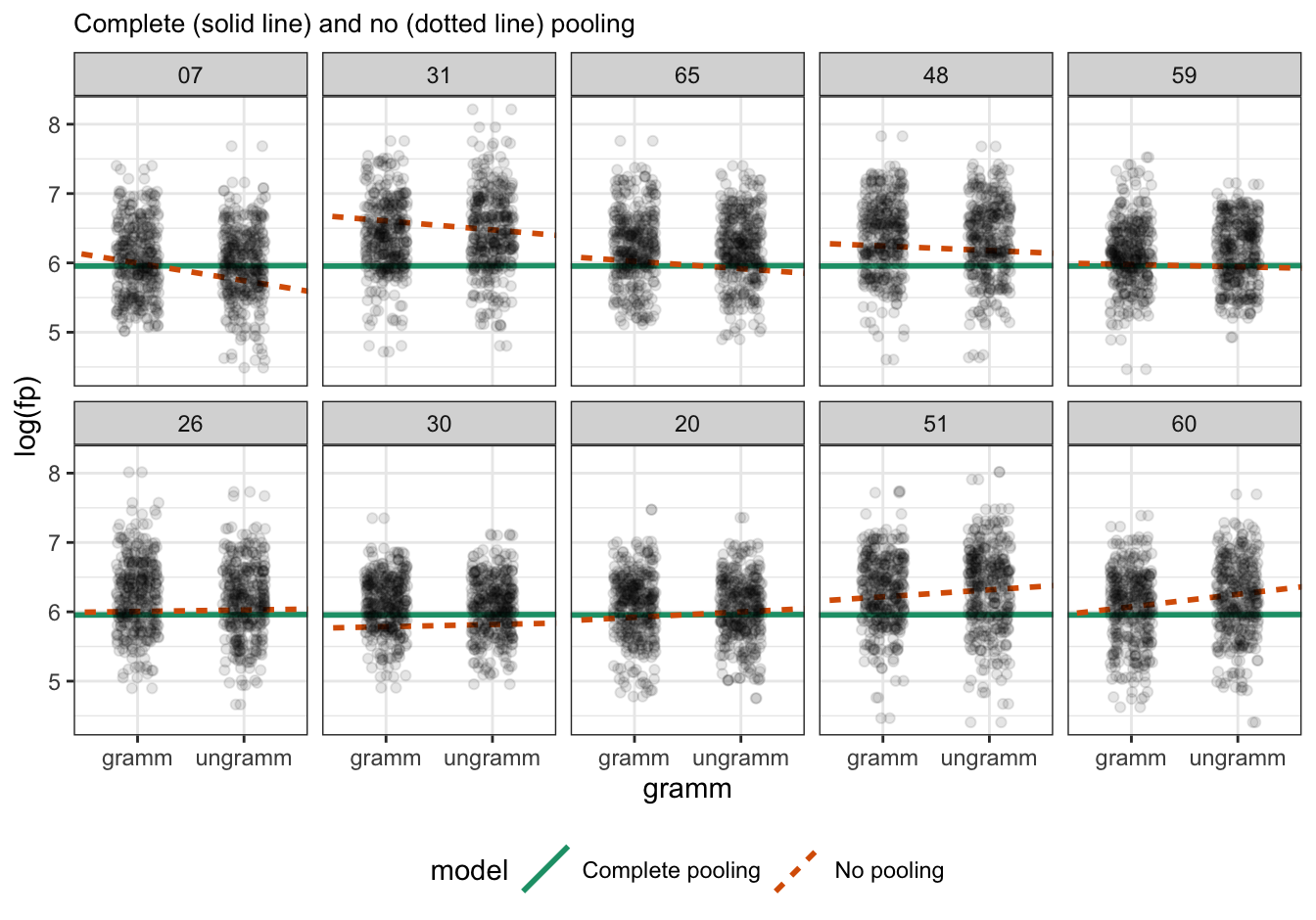
complete pooling (green solid line) and no pooling (orange dotted line) of grammaticality effects for 10 participants
- describe what you see in terms of intercept and slopes across the participants

Figure 12.1: Observations (black dots) with complete pooling regression line (solid green) and no pooling line (dotted orange) per 10 participants

12.4 Partial pooling: mixed models

13 Shrinkage

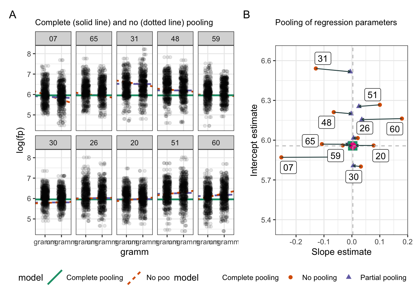
turns out the estimates are pulled towards the population-level estimates
- all the information in the model is taken into account when fitting varying intercepts and slopes

Figure 13.1: Elaine Benes learns about shrinkage of random effect estimates towards the population-level estimates

13.1 Shrinkage

Figure 13.2: Shrinkage of 10 participants

13.2 Centre of gravity

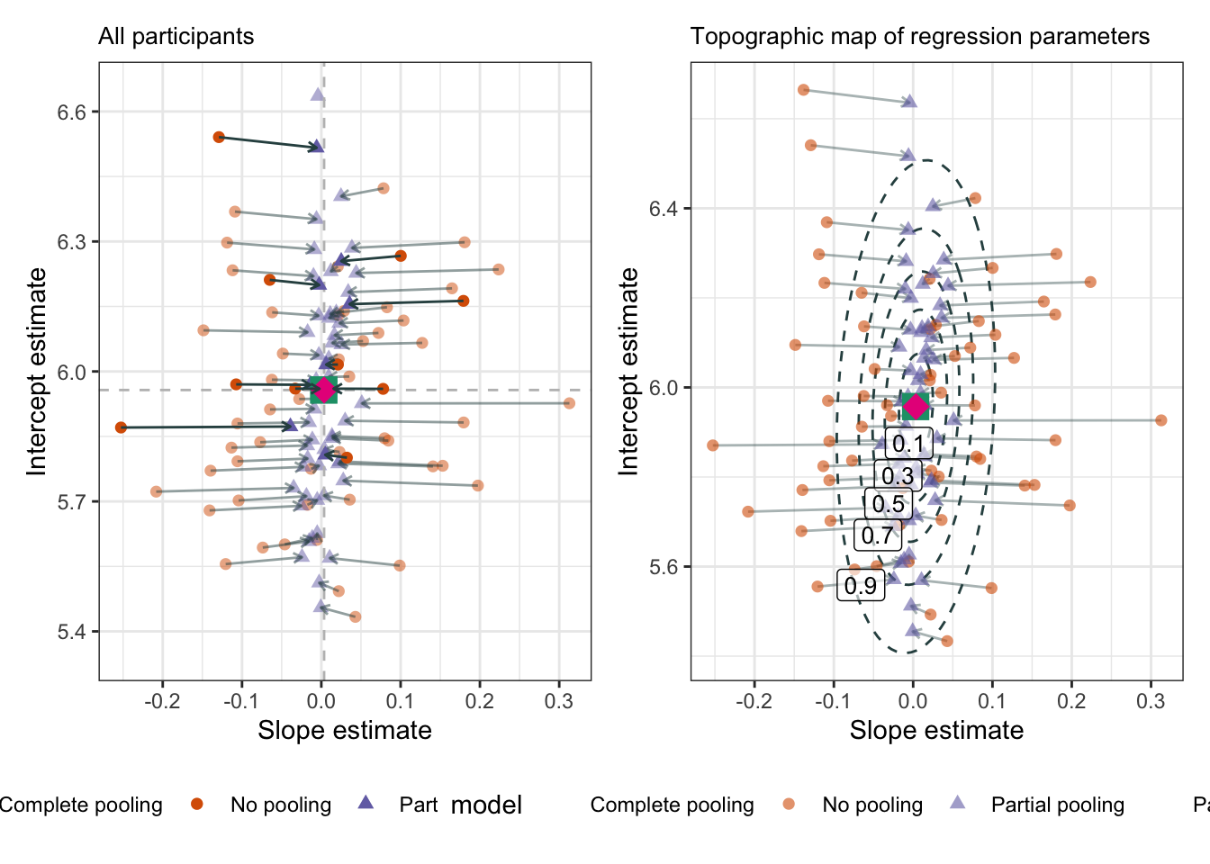
why are some points not being pulled directly to the ‘centre of gravity’?
- they’re being pulled to a higher confidence region

Figure 13.3: Shrinkage for all participants: each ellipsis represents a confidence level (really, a quantile: q1, q3, q5, q7, and q9); The inner ellipsis contains the centre 10% of the data, the outer ellipsis 90%

14 Why shrinkage?

with partial pooling, each random effect is liek a weighted average
- it takes into account the effect for one group level (e.g., one participant) and the population-level estiamtes
- the empirical effect for a group level is weighted by the number of observations
- so if one participant has fewer observations than another, then more weight is given to the population-level estimates, and vice versa
the implications (benefits) of this:
- imbalanced data are not a problem for linear mixed models
- the model can make predictions for unseen levels, i.e., it can generalise to new data

Learning objectives 🏁

Today we learned…

what linear mixed models are ✅
how to fit a random-intercepts model ✅
how to inspect and interpret a mixed effects model ✅

Important terms

Term	Definition	Equation/Code
linear mixed (effects) model	NA	NA

References

--- title: "Shrinkage and Partial Pooling" subtitle: "Shrinkage of random Complete, No, Partial Pooling" author: "Daniela Palleschi" institute: Humboldt-Universität zu Berlin # footer: "Lecture 1.1 - R und RStudio" lang: en date: "01/12/2024" date-modified: last-modified --- ::: {.callout-warning} # Under construction {.unnumbered .uncounted .unlisted} This chapter is not fully translated from bullet points (from my slides) to prose. This will happen eventually (hopefully by spring 2024). ::: This chapter presents figures from the [blog post](https://www.tjmahr.com/plotting-partial-pooling-in-mixed-effects-models/) "Plotting partial pooling in mixed-effects models" from Tristin Mahr (2017). You can also read Section 15.9 \'Shrinkage and Individual Differences' in @winter_statistics_2019 and Box 8.2 \'Broader Context: Shrinkage and Partial Pooling' in @sonderegger_regression_2023 for a short overview of the topics of shrinkage and partial pooling. We will be using the data from @biondo_yesterday_2022. # Learning Objectives {.unnumbered .unlisted} Today we will learn... - about no/complete/partial pooling - about shrinkage # Set-up {.unnumbered} ```{r} # suppress scientific notation options(scipen=999) ``` ## Load packages {.unnumbered} ```{r} # load libraries pacman::p_load( tidyverse, janitor, here, lmerTest) ``` ```{r} #| echo: false # set preferred ggplot2 theme theme_set(theme_bw() + theme(plot.title = element_text(size = 10))) ``` ```{r} lmer <- lmerTest::lmer ``` ```{r} #| echo: false # extra packages for the lecture notes/slides pacman::p_load( patchwork, knitr, kableExtra, googlesheets4, gt) # tell googlesheets4 we don't want private gs4_deauth() ``` ## Load data {.unnumbered} - data from @biondo_yesterday_2022 ```{r} df_biondo <- read_csv(here("data", "Biondo.Soilemezidi.Mancini_dataset_ET.csv"), locale = locale(encoding = "Latin1") ## for special characters in Spanish ) |> clean_names() |> mutate(gramm = ifelse(gramm == "0", "ungramm", "gramm")) |> mutate_if(is.character,as_factor) |> # all character variables as factors droplevels() |> filter(adv_type == "Deic") ``` ## Set contrasts ```{r} contrasts(df_biondo$verb_t) <- c(-0.5,+0.5) contrasts(df_biondo$gramm) <- c(-0.5,+0.5) contrasts(df_biondo$adv_type) <- c(-0.5,+0.5) ``` ```{r} #| output-location: column-fragment contrasts(df_biondo$verb_t) ``` ```{r} #| output-location: column-fragment contrasts(df_biondo$gramm) ``` ```{r} #| output-location: column-fragment contrasts(df_biondo$adv_type) ``` ## Run models - random-intercepts only ```{r} fit_fp_1 <- lmer(log(fp) ~ verb_t*gramm + (1 |sj) + (1|item), data = df_biondo, subset = roi == 4) ``` - by-item varying tense slopes ```{r} fit_fp_item <- lmerTest::lmer(log(fp) ~ verb_t*gramm + (1 |sj) + (1 + verb_t|item), data = df_biondo, subset = roi == 4) ``` # Pooling {.smaller} - do the random effects represent the exact average of participants? - below we see the mean logged first-pass reading time per participant (`mean`) and the by-participant intercepts from `fit_fp_1` and `fit_fp_item` - to understand what's happening, we first have to understand pooling ```{r} #| code-fold: true #| output-location: fragment sum_shrinkage <- df_biondo |> filter(roi == 4) |> summarise(mean = mean(log(fp), na.rm = T), .by = "sj") |> mutate(population_mean = mean(mean, na.rm = T)) |> left_join(coef(fit_fp_1)$sj["(Intercept)"] |> rownames_to_column(var = "sj")) |> rename(intercept_1 = `(Intercept)`) |> left_join(coef(fit_fp_item)$sj["(Intercept)"] |> rownames_to_column(var = "sj")) |> rename(intercept_item = `(Intercept)`) sum_shrinkage |> head() ``` ## No pooling {.smaller} :::: {.columns} ::: {.column width="100%"} - no pooling refers to separate regression lines fit e.g., per participant + each regression line is fit ignoring the population-level information + the intercepts are the true mean from each participant ::: ::: {.column width="50%"} ```{r} #| echo: false #| include: false df_no_pooling <- lmList(log(fp) ~ verb_t*gramm | sj, df_biondo, subset = roi == 4) %>% coef() %>% add_column(model = "No pooling") %>% # Subject IDs are stored as row-names. Make them an explicit column rownames_to_column("sj") %>% rename(intercept = `(Intercept)`) |> relocate(model) head(df_no_pooling) ``` ```{r} #| output-location: fragment head(df_no_pooling) ``` ::: ::: {.column width="50%"} ```{r} #| output-location: fragment sum_shrinkage |> head(6) ``` ::: :::: ## Complete pooling {.smaller} :::: {.columns} ::: {.column width="100%"} - complete pooling refers to ignoring grouping factors + i.e., fixed-effects only models (e.g., with `lm()` or `glm()`) + one regression line fit ignoring the individual-level information + the intercepts are the same as the population-level mean ::: ::: {.column width="50%"} ```{r} #| echo: false fit_pooled <- lm(log(fp) ~ verb_t*gramm, data = df_biondo, subset = roi == 4) # Repeat the intercept and slope terms for each participant df_pooled <- tibble( model = "Complete pooling", sj = unique(df_biondo$sj), intercept = coef(fit_pooled)[1], verb_t1 = coef(fit_pooled)[2], gramm1 = coef(fit_pooled)[3], `verb_t1:gramm1` = coef(fit_pooled)[4] ) ``` ```{r} #| output-location: fragment head(df_pooled) ``` ::: ::: {.column width="50%"} ```{r} #| output-location: fragment sum_shrinkage |> head(6) ``` ::: :::: ## Complete vs. no pooling :::: {.columns} ::: {.column width="40%"} - complete pooling (green solid line) and no pooling (orange dotted line) of grammaticality effects for 10 participants + describe what you see in terms of intercept and slopes across the participants ::: ::: {.column width="60%"} ```{r} #| echo: false # Join the raw data so we can use plot the points and the lines. df_models <- bind_rows(df_pooled, df_no_pooling) %>% left_join(df_biondo, by = "sj") # extract every 6th sj value ordered by verb_t slope sj_10 <- df_models |> filter(model == "No pooling") |> arrange(gramm1) |> mutate(sj = fct_reorder(sj, gramm1)) |> mutate(sj_slope = cur_group_id(), .by = sj, adv_sum = ifelse(verb_t == "Past", -0.5, 0.5)) |> slice(which(sj_slope %% 6 == 1)) |> distinct(sj) |> droplevels() |> select(sj) %>% unlist(use.names = FALSE) p_model_comparison <- df_models |> filter(sj %in% sj_10) |> mutate(sj = fct_reorder(sj, gramm1)) |> droplevels() |> ggplot() + aes(x = gramm, y = log(fp)) + labs(title = "Complete (solid line) and no (dotted line) pooling") + # Set the color mapping in this layer so the points don't get a color geom_abline( group = 1, linewidth = 1, aes(intercept = intercept - gramm1*1.5, slope = gramm1, color = model, linetype = model) ) + geom_point(alpha = .1, position = position_jitter(.2)) + facet_wrap("sj", nrow = 2) + # labs(x = xlab, y = ylab) + # scale_x_continuous(breaks = 0:4 * 2) + # Fix the color palette scale_color_brewer(palette = "Dark2") + theme(legend.position = "bottom") ``` ```{r} #| echo: false #| label: fig-no-complete #| fig-cap: "Observations (black dots) with complete pooling regression line (solid green) and no pooling line (dotted orange) per 10 participants" #| fig-asp: .7 p_model_comparison ``` ::: :::: ## Partial pooling: mixed models ```{r} #| echo: false m <- lmer(log(fp) ~ 1 + gramm*verb_t + (1 + gramm | sj), df_biondo, subset = roi == 4) # arm::display(m) # summary(m) ``` ```{r} #| echo: false #| include: false # Make a dataframe with the fitted effects df_partial_pooling <- coef(m)[["sj"]] %>% rownames_to_column("sj") %>% as_tibble() %>% rename(intercept = `(Intercept)`) %>% add_column(model = "Partial pooling") head(df_partial_pooling) ``` ```{r} #| echo: false # Update the previous plot with a dataframe of all three models’ estimates. df_models <- bind_rows(df_pooled, df_no_pooling, df_partial_pooling) %>% left_join(df_biondo, by = "sj") |> arrange(gramm1) |> mutate(sj = fct_reorder(sj, gramm1)) |> mutate(sj_slope = cur_group_id(), .by = sj, tense_sum = ifelse(verb_t == "Past", -0.5, 0.5)) |> # slice(which(sj_slope %% 6 == 1)) filter(sj %in% sj_10) # Replace the data-set of the last plot fig_pooling <- p_model_comparison %+% df_models ``` # Shrinkage - turns out the estimates are pulled towards the population-level estimates + all the information in the model is taken into account when fitting varying intercepts and slopes ```{r} #| echo: false #| label: fig-shrinks #| fig-cap: Elaine Benes learns about shrinkage of random effect estimates towards the population-level estimates knitr::include_graphics(here::here( "media", "seinfeld_shrinks.png" )) ``` ```{r} #| echo: false #| include: false df_biondo |> filter(roi == 4) |> mutate(mean_sj = mean(fp, na.rm = T), .by = c(sj)) |> arrange(mean_sj) |> # mutate(sj_order = cur_group_id(), .by = sj) |> # slice(sj %% 12 == 1) # slice(sj_order %% 12 == 1) droplevels() |> ggplot() + aes(x = gramm, y = fp) + facet_wrap(~fct_reorder(sj, mean_sj)) + stat_smooth(aes(group = 1), method = "lm", se = FALSE) + # Put the points on top of lines geom_point() + labs(x = "Grammaticality", y = "FP (ms)") # We also need to help the x-axis, so it doesn't # create gridlines/ticks on 2.5 days # scale_x_discrete(breaks = c(-0.5, 0.5)) #> `geom_smooth()` using formula 'y ~ x' ``` ## Shrinkage ```{r} #| echo: false # Also visualize the point for the fixed effects df_fixef <- tibble( model = "Partial pooling (average)", intercept = fixef(m)[1], gramm1 = fixef(m)[2] ) # Complete pooling / fixed effects are center of gravity in the plot df_gravity <- df_pooled %>% distinct(model, intercept, gramm1) %>% bind_rows(df_fixef) # df_gravity # # A tibble: 2 × 3 # model intercept gramm1 # <chr> <dbl> <dbl> # 1 Complete pooling 5.96 0.00310 # 2 Partial pooling (average) 5.96 0.00350 df_pulled <- bind_rows(df_no_pooling, df_partial_pooling) fig_shrink_10 <- ggplot(df_pulled |> filter(sj %in% sj_10)) + aes(y = intercept, x = gramm1, color = model, shape = model) + geom_point(size = 2) + geom_point( data = df_gravity, size = 5, # Prevent size-5 point from showing in legend keys show.legend = FALSE ) + # add dashed lines to indicate partial pooling intercept and slope geom_vline(linetype = "dashed", colour = "grey", aes(xintercept = fixef(m)[2]) ) + geom_hline( linetype = "dashed", colour = "grey", aes(yintercept = fixef(m)[1]) ) + # Draw an arrow connecting the observations between models geom_path(colour = "darkslategrey", aes(group = sj, color = NULL), arrow = arrow(length = unit(.02, "npc")), show.legend = FALSE ) + # Use ggrepel to jitter the labels away from the points ggrepel::geom_label_repel( data = df_no_pooling |> filter(sj %in% sj_10), show.legend = FALSE, aes(label = sj, color = NULL) ) + scale_y_continuous(breaks = c(5.4,5.7,6,6.3,6.6), limits = c(5.35, 6.65)) + # Don't forget 373 # ggrepel::geom_text_repel( # aes(label = sj, color = NULL), # data = filter(df_partial_pooling), # show.legend = FALSE # ) + theme( legend.position = "bottom" ) + labs( title = "Pooling of regression parameters", x = "Slope estimate", y = "Intercept estimate" ) + scale_shape_manual(values = c(15:18)) + scale_color_brewer(palette = "Dark2") ``` ```{r} #| echo: false "%nin%" <- function(x, table) match(x, table, nomatch = 0L) == 0L fig_shrink_all <- ggplot(df_pulled |> filter(sj %nin% sj_10)) + aes(y = intercept, x = gramm1, color = model, shape = model) + # faded for all the other points geom_point( alpha = 0.5,size = 2) + geom_point( alpha = 0.5, data = df_gravity, size = 5, # Prevent size-5 point from showing in legend keys show.legend = FALSE ) + # add dashed lines to indicate partial pooling intercept and slope geom_vline(linetype = "dashed", colour = "grey", aes(xintercept = fixef(m)[2]) ) + geom_hline( linetype = "dashed", colour = "grey", aes(yintercept = fixef(m)[1]) ) + # Draw an arrow connecting the observations between models geom_path(colour = "darkslategrey", alpha = 0.5, aes(group = sj, color = NULL), arrow = arrow(length = unit(.02, "npc")), show.legend = FALSE ) + # overlay our 10 points geom_point(data = df_pulled |> filter(sj %in% sj_10), size = 2) + geom_point( data = df_gravity, size = 5, # Prevent size-5 point from showing in legend keys show.legend = FALSE ) + # Draw an arrow connecting the observations between models geom_path(colour = "darkslategrey", data = df_pulled |> filter(sj %in% sj_10), aes(group = sj, color = NULL), arrow = arrow(length = unit(.02, "npc")), show.legend = FALSE ) + scale_y_continuous(breaks = c(5.4,5.7,6,6.3,6.6), limits = c(5.35, 6.65)) + # Use ggrepel to jitter the labels away from the points # ggrepel::geom_label_repel( # data = df_no_pooling |> filter(sj %in% sj_10), # show.legend = FALSE, # aes(label = sj, color = NULL) # ) + # Don't forget 373 # ggrepel::geom_text_repel( # aes(label = sj, color = NULL), # data = filter(df_partial_pooling), # show.legend = FALSE # ) + theme( legend.position = "bottom" ) + labs( title = "All participants", x = "Slope estimate", y = "Intercept estimate" ) + scale_shape_manual(values = c(15:18)) + scale_color_brewer(palette = "Dark2") ``` ```{r, fig.dpi=600} #| echo: false #| label: fig-pooling #| fig-cap: Shrinkage of 10 participants #| out-width: "100%" fig_pooling + fig_shrink_10 + plot_annotation(tag_levels = "A") + plot_layout(widths = c(3,2)) ``` ## Centre of gravity - why are some points not being pulled directly to the 'centre of gravity'? + they're being pulled to a higher confidence region ```{r} #| echo: false #| include: false ## Extract the matrix cov_mat <- VarCorr(m)[["sj"]] # Strip off some details so that just the useful part is printed attr(cov_mat, "stddev") <- NULL attr(cov_mat, "correlation") <- NULL cov_mat # (Intercept) gramm1 # (Intercept) 0.065744230 0.001637183 # gramm1 0.001637183 0.002165894 ``` ```{r} #| echo: false #| include: false library(ellipse) #> #> Attaching package: 'ellipse' #> The following object is masked from 'package:graphics': #> #> pairs # Helper function to make a data-frame of ellipse points that # includes the level as a column make_ellipse <- function(cov_mat, center, level) { ellipse(cov_mat, centre = center, level = level) %>% as.data.frame() %>% add_column(level = level) %>% as_tibble() } center <- fixef(m) levels <- c(.1, .3, .5, .7, .9) # Create an ellipse dataframe for each of the levels defined # above and combine them df_ellipse <- levels %>% lapply( function(x) make_ellipse(cov_mat, center, level = x) ) %>% bind_rows() %>% rename(intercept = `(Intercept)`) df_ellipse #> # A tibble: 500 × 3 #> Intercept Slope_Days level #> <dbl> <dbl> <dbl> #> 1 261. 12.4 0.1 #> 2 260. 12.6 0.1 #> 3 260. 12.7 0.1 #> 4 259. 12.8 0.1 #> 5 258. 12.8 0.1 #> 6 258. 12.9 0.1 #> 7 257. 13.0 0.1 #> 8 257. 13.0 0.1 #> 9 256. 13.1 0.1 #> 10 255. 13.1 0.1 #> # … with 490 more rows ``` ```{r} #| echo: false #| include: false # Euclidean distance contour_dist <- function(xs, ys, center_x, center_y) { x_diff <- (center_x - xs) ^ 2 y_diff <- (center_y - ys) ^ 2 sqrt(x_diff + y_diff) } # Find the point to label in each ellipse. df_label_locations <- df_ellipse %>% group_by(level) %>% filter( intercept < quantile(intercept, .25), gramm1 < quantile(gramm1, .25) ) %>% # Compute distance from center. mutate( dist = contour_dist(intercept, gramm1, fixef(m)[1], fixef(m)[3]) ) %>% # Keep smallest values. top_n(-1, wt = dist) %>% ungroup() fig_ellipses <- ggplot(df_pulled) + aes(y = intercept, x = gramm1, color = model, shape = model) + # Draw contour lines from the distribution of effects geom_path(colour = "darkslategrey", aes(group = level, color = NULL, shape = NULL), data = df_ellipse, linetype = "dashed", color = "grey40" ) + geom_path(colour = "darkslategrey", aes(group = sj, color = NULL), arrow = arrow(length = unit(.02, "npc")), show.legend = FALSE, alpha = .4 ) + geom_point(size = 2, alpha = .6) + theme( legend.position = "bottom" ) + ggtitle("Topographic map of regression parameters") + ylab("Intercept estimate") + xlab("Slope estimate") + scale_color_brewer(palette = "Dark2") + scale_shape_manual(values = c(15:18)) + geom_point( aes(shape = model), data = df_gravity, size = 5, show.legend = FALSE ) # geom_text( # aes(label = level, color = NULL, shape = NULL), # data = df_label_locations, # nudge_x = .5, # nudge_y = .8, # size = 3.5, # color = "grey40" # ) fig_ellipses + coord_cartesian( ylim = range(df_pulled$intercept), xlim = range(df_pulled$gramm1), expand = TRUE ) ``` ```{r} #| include: false #| echo: false # Euclidean distance contour_dist <- function(xs, ys, center_x, center_y) { x_diff <- (center_x - xs) ^ 2 y_diff <- (center_y - ys) ^ 2 sqrt(x_diff + y_diff) } # Find the point to label in each ellipse. df_label_locations <- df_ellipse %>% group_by(level) %>% filter( intercept < quantile(intercept, .25), gramm1 < quantile(gramm1, .25) ) %>% # Compute distance from center. mutate( dist = contour_dist(intercept, gramm1, fixef(m)[1], fixef(m)[2]) ) %>% # Keep smallest values. top_n(-1, wt = dist) %>% ungroup() # Tweak the last plot one more time! fig_ellipses <- fig_ellipses + geom_label( aes(label = level, color = "NULL", shape = NULL), data = df_label_locations, nudge_y = .005, nudge_x = .008, size = 3.5, color = "black", alpha = .6 ) ``` ```{r} #| echo: false #| label: fig-ellipses #| fig-cap: "Shrinkage for all participants: each ellipsis represents a confidence level (really, a quantile: q1, q3, q5, q7, and q9); The inner ellipsis contains the centre 10% of the data, the outer ellipsis 90%" fig_shrink_all + fig_ellipses ``` # Why shrinkage? - with partial pooling, each random effect is liek a weighted average + it takes into account the effect for one group level (e.g., one participant) *and* the population-level estiamtes + the empirical effect for a group level is weighted by the number of observations + so if one participant has fewer observations than another, then more weight is given to the population-level estimates, and vice versa - the implications (benefits) of this: + imbalanced data are not a problem for linear mixed models + the model can make predictions for unseen levels, i.e., it can generalise to new data # Learning objectives 🏁 {.unnumbered .unlisted .uncounted} Today we learned... - what linear mixed models are ✅ - how to fit a random-intercepts model ✅ - how to inspect and interpret a mixed effects model ✅ # Important terms {.unnumbered .smaller .uncounted} ```{r} #| echo: false content <- googlesheets4::read_sheet("https://docs.google.com/spreadsheets/d/17CqdxKL9lyy-PbTB2ZnfWNWs4oV--CcBvrqlh_aEPGQ/edit?usp=sharing") content |> filter(`Lecture topic` == "08 - LMMs 1: random intercepts") |> select(-`Lecture topic`) |> gt() ``` # References {.unlisted .unnumbered visibility="uncounted"} ::: {#refs custom-style="Bibliography"} :::

References

Biondo, N., Soilemezidi, M., & Mancini, S. (2022). Yesterday is history, tomorrow is a mystery: An eye-tracking investigation of the processing of past and future time reference during sentence reading. Journal of Experimental Psychology: Learning, Memory, and Cognition, 48(7), 1001–1018. https://doi.org/10.1037/xlm0001053
Sonderegger, M. (2023). Regression Modeling for Linguistic Data.
Winter, B. (2019). Statistics for Linguists: An Introduction Using R. In Statistics for Linguists: An Introduction Using R. Routledge. https://doi.org/10.4324/9781315165547