6  Logistic regression

Regression for Linguists

Author

Affiliation

Daniela Palleschi

Humboldt-Universität zu Berlin

This lecture jumps to chapter 12 'Genearlised Lienar Models 1: Logistic Regression’ (Winter, 2019). We’re skipping a few chapters, which I encourage you to go through on your own. However, they cover topics that you presumably have covered in previous courses (namely significance testing, t-values and p-values).

Learning Objectives

Today we will learn…

• how to model binomial data with logistic regression
• how to interpret log-odds and odds ratio

Set-up environment

# suppress scientific notation
options(scipen=999)
options(pillar.sigfig = 5)

library(broman)
# function to format p-values
format_pval <- function(x){
  if (x < .001) return(paste('<', '.001'))
  if (x < .01) return(paste('<', '.01'))
  if (x < .05) return(paste('<', '.05'))
  paste('=', myround(x, 3))  # if above .05, print p-value to 3 decimalp points
}

We’ll also need to load in our required packages. Hopefully you’ve already install the required packages (if not, go to Chapter 3).

# load libraries
pacman::p_load(
               tidyverse,
               here,
               broom,
               lme4,
               janitor,
               languageR)

# set preferred ggplot2 theme
theme_set(theme_bw() + theme(plot.title = element_text(size = 10)))

6.1 Generalised linear models

Logistic regression is a type of genearlised linear model (GLM), and is used to model binomial response data. Whereas continuous response variables, such as reaction times, assume a normal distribution (a.k.a., a Gaussian distribution), logistic regression assumes a binomial distribution (a.k.a., Bernoulli distribution). These are formalised in equations \(\ref{eq-normal}\), where \(\mu\) and \(\sigma\) correspond to the mean and standard deviation, and \(\ref{eq-binomial}\), where \(N\) and \(p\) refer to the number of trials and the probability of \(y\) being \(1\) or \(0\).

\[\begin{align} y &\sim Normal(\mu,\sigma) \label{eq-normal} \\ y &\sim binomial(N = 1, p) \label{eq-binomial} \end{align}\]

Don’t stress about this for now, I find the math behind everything will start to make more sense the more often you see it. However, some math is necessary in order to understand the output of our models, namely the relation between probabilities, odds, and log odds.

6.1.1 Log-odds, odds ratio, and probabilities

In logistic regression, we the probability (\(p\)) of observing one outcome or another as a function of a predictor variable. In linguistic research, these outcomes could be the absence or presence of some phenomenon (pause, schwa, etc.) or button responses (yes/no, accept/reject). In logistic regression, we describe the probability, odds, or log-odds of a particular outcome over another.

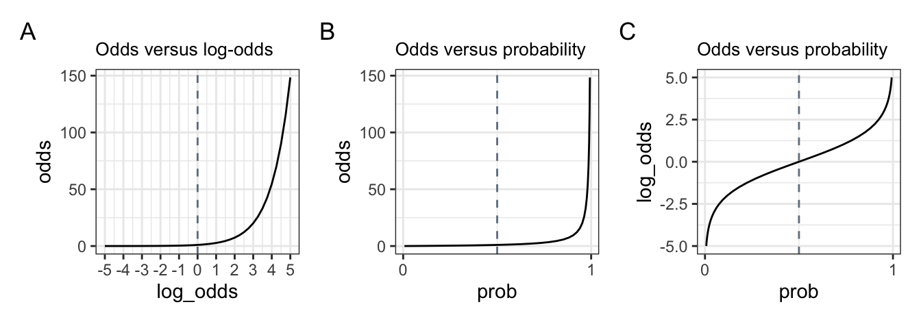
Probability is quite intuitive, and ranges from 0 (no chance) to 1 (certain). A 50% chance corresponds to a probability of 0.5. You’re also likely familiar with odds, which can range from 0 to infinity. Odds are often used in betting, such as the odds that I’ll win are 2:1, which corresponds to \(\frac{2}{1} = 2\) in favour of my winning. Conversely, the odds that you’ll win are 1:2, corresponding to \(\frac{1}{2} = 0.5\), meaning it’s less likely that you’ll win compared to you losing. If the odds are even, then: \(\frac{1}{1} = 1\). So, odds of 1 correspond to a probability of 0.5. Log-odds are just the logarithmically-transformed odds: \(log(2) =\) 0.6931472; \(log(0.5) =\) -0.6931472; \(log(1) =\) 0. Probability can also be computed using the odds, as shown in \(\ref{eq-odds}\): \(\frac{2}{1+2} =\) 0.6666667; \(\frac{1}{1+1} =\) 0.5; \(\frac{0.5}{1+0.5} =\) 0.3333333.

We can get the probability from a log odds value using plogis(), which performs the following calculation:

\[\begin{equation} p = \frac{exp(log\;odds)}{1 + exp(log\;odds)} = \frac{odds}{1 + odds} \label{eq-odds} \end{equation}\]

Table 6.1 gives an example of how the three relate to each other. The grey cells are all where chances re 50/50, with increasingly more likely (green) or less likely (red) values/

Table 6.1: Comparison of different values of probabilities/odds/log-odds

name	1	2	3	4	5	6	7	8	9
prob	0.0066929	0.0229774	0.0758582	0.2227001	0.5	0.7772999	0.9241418	0.9770226	0.9933071
odds	0.0067379	0.0235177	0.0820850	0.2865048	1.0	3.4903430	12.1824940	42.5210820	148.4131591
log_odds	-5.0000000	-3.7500000	-2.5000000	-1.2500000	0.0	1.2500000	2.5000000	3.7500000	5.0000000

This relationship is demonstrated in Figure 6.1. Take your time to really understand these plots, as it will help understand the output of our models.

Figure 6.1: Relationship between probability, odds, and log-odds

6.2 Logistic regression

I find the more we talk about the math behind the models before even running a model, the more overwhelmed we become. So, let’s run our first logistic regression and then dissect it to understand it. Most relevant to the output of a logistic regression model is Figure 6.1 C, as the model will output log-odds, and we most likely want to interpret them in terms of probabilities.

We’ll use a dataset from Biondo et al. (2022), an eye-tracking reading study exploring the processing of adverb-tense concord in Spanish past and future tenses. Participants read sentences that began with a temporal adverb (e.g., yesterday/tomorrow), and had a verb marked with the congruent or incongruent tense (past/future). We will look at the measure regression in at the verb region.

Let’s start by loading in the data:

df_tense <-
  read_csv(here("data", "Biondo.Soilemezidi.Mancini_dataset_ET.csv"),
           locale = locale(encoding = "Latin1") # for special characters in Spanish
           ) |> 
  mutate(gramm = ifelse(gramm == "0", "ungramm", "gramm")) |> 
  clean_names() |> 
  filter(roi == 4,
         adv_type == "Deic")

6.2.1 EDA

And conducting a quick EDA: print summaries and plot the response variables.

head(df_tense)

# A tibble: 6 × 13
  sj     item adv_type adv_t  verb_t gramm     roi label    fp    gp    tt    ri
  <chr> <dbl> <chr>    <chr>  <chr>  <chr>   <dbl> <chr> <dbl> <dbl> <dbl> <dbl>
1 1        54 Deic     Past   Past   gramm       4 enca…  1027  1027  1027     0
2 1         4 Deic     Future Future gramm       4 cole…   562   562  1337     1
3 1        62 Deic     Past   Past   gramm       4 esqu…   293  1664  1141     0
4 1        96 Deic     Future Past   ungramm     4 cons…   713  1963  1868     0
5 1        52 Deic     Past   Past   gramm       4 desa…   890   890  1707     1
6 1        90 Deic     Future Past   ungramm     4 dece…   962   962   962     0
# ℹ 1 more variable: ro <dbl>

Let’s look at only our binomial dependent variables, regression in (ri) and regression out (ro). For each variable, 1 indicates a regression in/out, 0 indicates there was no regression in/out.

df_tense |> 
  select(roi, ri, ro) |> 
  summary()

      roi          ri               ro         
 Min.   :4   Min.   :0.0000   Min.   :0.00000  
 1st Qu.:4   1st Qu.:0.0000   1st Qu.:0.00000  
 Median :4   Median :0.0000   Median :0.00000  
 Mean   :4   Mean   :0.2248   Mean   :0.08169  
 3rd Qu.:4   3rd Qu.:0.0000   3rd Qu.:0.00000  
 Max.   :4   Max.   :1.0000   Max.   :1.00000  
             NA's   :45       NA's   :45       

Let’s plot out our dependent variable of interest: regression in.

# make grammaticality a factor
df_tense |> 
  mutate(gramm = as_factor(gramm)) 

# A tibble: 3,840 × 13
   sj     item adv_type adv_t  verb_t gramm    roi label    fp    gp    tt    ri
   <chr> <dbl> <chr>    <chr>  <chr>  <fct>  <dbl> <chr> <dbl> <dbl> <dbl> <dbl>
 1 1        54 Deic     Past   Past   gramm      4 enca…  1027  1027  1027     0
 2 1         4 Deic     Future Future gramm      4 cole…   562   562  1337     1
 3 1        62 Deic     Past   Past   gramm      4 esqu…   293  1664  1141     0
 4 1        96 Deic     Future Past   ungra…     4 cons…   713  1963  1868     0
 5 1        52 Deic     Past   Past   gramm      4 desa…   890   890  1707     1
 6 1        90 Deic     Future Past   ungra…     4 dece…   962   962   962     0
 7 1         8 Deic     Future Future gramm      4 evid…   718   718   718     0
 8 1         9 Deic     Future Future gramm      4 excu…  1453  1453  1453     0
 9 1        56 Deic     Past   Past   gramm      4 equi…   769   769   769     0
10 1        11 Deic     Future Future gramm      4 cena…   778   778   778     0
# ℹ 3,830 more rows
# ℹ 1 more variable: ro <dbl>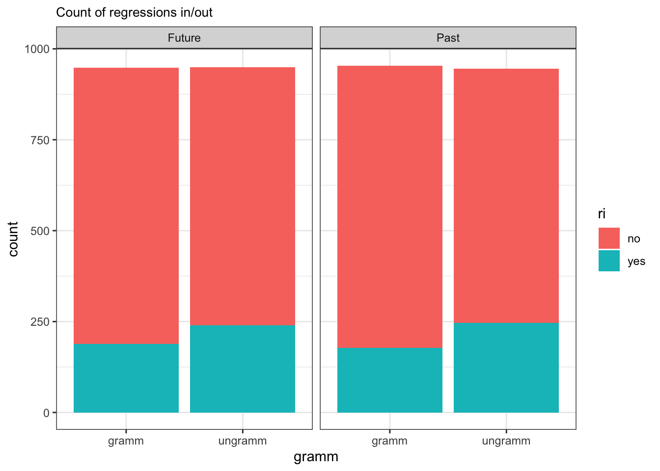

It looks like there are more regressions in for the grammatical versus ungrammatical conditions in both the future and past tenses. There doesn’t seem to be a large difference between the two tenses in overall regressions in, nor in the effect of grammaticality on the proportion of regressions in. We can also see that it was more likely overall for there to not be a regression in (versus for there to be a regression in).

6.2.2 Model

Now let’s run our model. Verb tense and grammaticality are each two-level factors, so we’ll want to set sum coding for each of them. Let’s set past and grammatical to \(-0.5\), and future and ungrammatical to +0.5.

df_tense$verb_t <- as.factor(df_tense$verb_t)
levels(df_tense$verb_t)

[1] "Future" "Past"  

contrasts(df_tense$verb_t) <- c(+0.5, -0.5)
contrasts(df_tense$verb_t)

       [,1]
Future  0.5
Past   -0.5

df_tense$gramm <- as.factor(df_tense$gramm)
levels(df_tense$gramm)

[1] "gramm"   "ungramm"

contrasts(df_tense$gramm) <- c(-0.5, +0.5)
contrasts(df_tense$gramm)

        [,1]
gramm   -0.5
ungramm  0.5

Now that we’ve set our contrasts (if you have continuous predictors, you would centre and potentially standardise them instead), we can fit our model. We use the glm() function to fit a genearlised linear model, and use the argument family = "binomial" to indicate our data are binomial.

fit_tense_ri <-
  glm(ri ~ verb_t*gramm,
    data = df_tense,
    family = "binomial")

What do our coefficients look like?

tidy(fit_tense_ri) %>%
  mutate(p.value = as.numeric(p.value)) |> 
  mutate(p.value = round(p.value*4,10)
         ) |> 
  knitr::kable() |> 
  kableExtra::kable_styling()

term	estimate	std.error	statistic	p.value
(Intercept)	-1.2472175	0.0392027	-31.8146220	0.0000000
verb_t1	0.0209637	0.0784053	0.2673755	3.1567201
gramm1	0.3668992	0.0784053	4.6795205	0.0000115
verb_t1:gramm1	-0.1197221	0.1568106	-0.7634823	1.7807033

Let’s first consider the estimates. The intercept is negative, meaning it is below 0. Verb tense is positive, meaning that there are more regressions in for the future compared to the past, holding grammaticality constant. Grammaticality is positive, meaning that there were more regressions in for the ungrammatical than grammatical conditions. But what does zero mean here? Logistic regression gives the estimates in log-odds. This means that a value of 0 means there is an equal probability of a regression in or out for both conditions (as in (tab-odds?)), i.e., the slope is flat (or not significantly different from 0). How can we convert our log-odds estimates to something more interpretable, like probabilities? Recall the equation in \(\ref{eq-odds}\), which would require a lot of typing. Luckily, we can just use the plogis() function, which takes a log-odds value and spits out the corresponding probability. We can also just use the exp() function to get the odds ratio from the log-odds.

plogis(-1.23) # intercept prob

[1] 0.2261814

plogis(0.0277) # tense prob

[1] 0.5069246

exp(-1.23) # intercept odds

[1] 0.2922926

exp(0.0277) # tense odds

[1] 1.028087

This is great, but a bit tedious. We can also just feed a tibble column through the plogis() and exp() functions to print a table with the relevant probabilities and odds.

tidy(fit_tense_ri) %>%
  mutate(p.value = round(p.value*4,10),
         prob = plogis(estimate),
         odds = exp(estimate)
         ) |> 
  mutate_if(is.numeric, round, 4) |> 
  knitr::kable() |> 
  kableExtra::kable_styling()

term	estimate	std.error	statistic	p.value	prob	odds
(Intercept)	-1.2472	0.0392	-31.8146	0.0000	0.2232	0.2873
verb_t1	0.0210	0.0784	0.2674	3.1567	0.5052	1.0212
gramm1	0.3669	0.0784	4.6795	0.0000	0.5907	1.4433
verb_t1:gramm1	-0.1197	0.1568	-0.7635	1.7807	0.4701	0.8872

We see that the odds of the future tense have a regression in versus the past tense is ~1, with the corresponding probability of 0.51. Unsuprisingly, we see this p-value indicates this effect was not significant (p > .05), and the z-value (note: not t-value!) is also low.

z-values

z-values correspond to the estimate divided by the standard error. It’s interpretation is similar to that of the t-value: a z-value of ~2 or higher will likely have a p-value below 0.05.

The interaction term is negative, what does this mean? We can interpret this as indicating that the effect of congruence is different in either level of tense. These effects are often more easily interpreted with a visualisation, e.g., using the plot_model() function from the sjPlot package. This effect is not significant, however.

sjPlot::plot_model(fit_tense_ri, 
                   type = "eff", 
                   terms = c("gramm", "verb_t")) + 
  geom_line(position = position_dodge(0.1))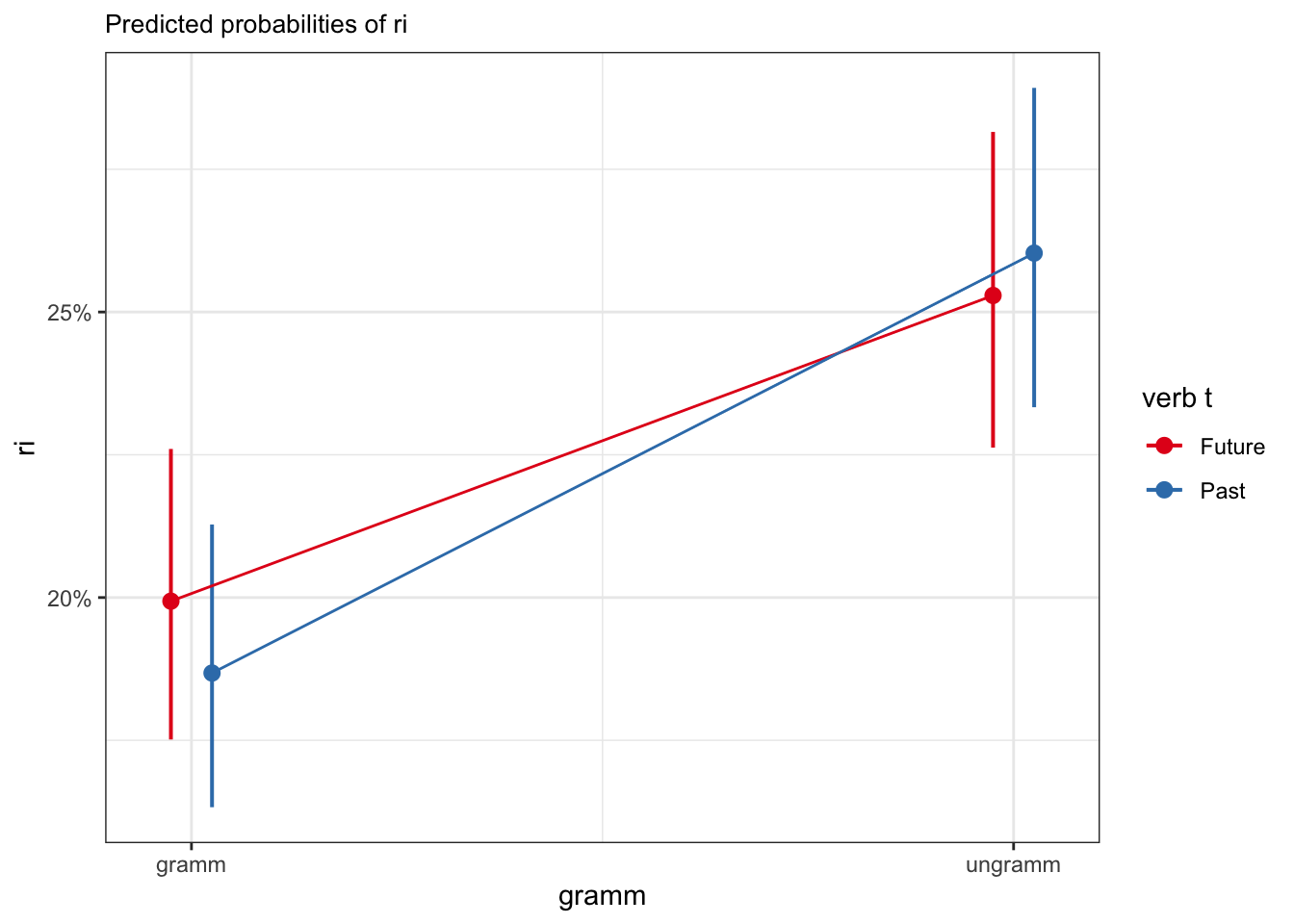

Figure 6.2: Interaction plot of

We can also use the predict() function to extract the predicted values for each condition. We could just simply print the predicted values (predict(fit_tense_ri)), append the predicted values to the data frame

# make sure dataset is the same length as the model data
df_tense_v <-
  df_tense |> 
  filter(roi == "4") |> 
  drop_na(ri)

# append model estimates
augment(fit_tense_ri, data = df_tense_v) |> 
  distinct(verb_t, gramm, .keep_all = T) |>
  arrange(verb_t) |>  
  select(verb_t, gramm, .fitted)

# A tibble: 4 × 3
  verb_t gramm   .fitted
  <fct>  <fct>     <dbl>
1 Future gramm   -1.3903
2 Future ungramm -1.0832
3 Past   gramm   -1.4711
4 Past   ungramm -1.0443

Or we could create a list of the unique conditions.

df_sim <-
    tibble(
    verb_t = rep(c('Past', 'Future'), each = 2),
    gramm = rep(c('0', '1'), times = 2))

# alternatively, just extract the relevant factor levels from your datafram
df_sim <-
  df_tense |> 
  arrange(verb_t) |> 
  distinct(verb_t, gramm) 

# and add predicted values
df_sim$fit <- num(predict(fit_tense_ri, df_sim), digits = 5)

df_sim

# A tibble: 4 × 3
  verb_t gramm         fit
  <fct>  <fct>   <num:.5!>
1 Future gramm    -1.39025
2 Future ungramm  -1.08322
3 Past   gramm    -1.47108
4 Past   ungramm  -1.04432

And now if we look at the predicted log-odds values for the future and past tenses:

df_sim |> 
  summarise(
    mean_tense = mean(fit),
    .by = verb_t)

# A tibble: 2 × 2
  verb_t mean_tense
  <fct>   <num:.5!>
1 Future   -1.23674
2 Past     -1.25770

What is the difference between these two numbers (in our model summary)?

df_sim |> 
  summarise(
    mean_tense = mean(fit),
    .by = gramm)

# A tibble: 2 × 2
  gramm   mean_tense
  <fct>    <num:.5!>
1 gramm     -1.43067
2 ungramm   -1.06377

What is the difference between these two numbers (in our model summary)?

So, our slopes for verb_t and gramm correspond to the predicted difference between the two levels of each factor.

6.3 Interpreting our coefficients

What do our coefficient estimates reflect, though? Let’s remind ourselves of the rate of regressions in at the verb region:

df_tense |> 
  filter(roi == "4") |> 
  drop_na(ri) |> 
  summary()

      sj                 item          adv_type            adv_t          
 Length:3795        Min.   :  1.00   Length:3795        Length:3795       
 Class :character   1st Qu.: 25.00   Class :character   Class :character  
 Mode  :character   Median : 52.00   Mode  :character   Mode  :character  
                    Mean   : 50.91                                        
                    3rd Qu.: 78.00                                        
                    Max.   :101.00                                        
    verb_t         gramm           roi       label                 fp        
 Future:1897   gramm  :1901   Min.   :4   Length:3795        Min.   :  81.0  
 Past  :1898   ungramm:1894   1st Qu.:4   Class :character   1st Qu.: 266.0  
                              Median :4   Mode  :character   Median : 371.0  
                              Mean   :4                      Mean   : 440.5  
                              3rd Qu.:4                      3rd Qu.: 535.0  
                              Max.   :4                      Max.   :2833.0  
       gp             tt               ri               ro         
 Min.   :  87   Min.   :  90.0   Min.   :0.0000   Min.   :0.00000  
 1st Qu.: 285   1st Qu.: 326.5   1st Qu.:0.0000   1st Qu.:0.00000  
 Median : 405   Median : 493.0   Median :0.0000   Median :0.00000  
 Mean   : 510   Mean   : 607.4   Mean   :0.2248   Mean   :0.08169  
 3rd Qu.: 606   3rd Qu.: 747.0   3rd Qu.:0.0000   3rd Qu.:0.00000  
 Max.   :3877   Max.   :3936.0   Max.   :1.0000   Max.   :1.00000  

ptab_gramm <-
  df_tense |> 
  filter(roi == "4") |> 
  drop_na(ri) |> 
  select(gramm, ri) |> 
  table() |> 
  prop.table()

ptab_tense <-
  df_tense |> 
  filter(roi == "4") |> 
  drop_na(ri) |> 
  select(verb_t, ri) |> 
  table() |> 
  prop.table()

df_tense |> 
  filter(roi == "4") |> 
  drop_na(ri) |> 
  tabyl(gramm, ri, verb_t) |> 
  adorn_percentages() |> 
  adorn_totals()

$Future
   gramm         0         1
   gramm 0.8006329 0.1993671
 ungramm 0.7471022 0.2528978
   Total 1.5477351 0.4522649

$Past
   gramm         0         1
   gramm 0.8132214 0.1867786
 ungramm 0.7396825 0.2603175
   Total 1.5529039 0.4470961

We want to measure how much more likely a regression in (y = 1) is for ungrammatical conditions (x = 1) than in grammatical conditions (x = 0). Si we want to calculate the odds of a regression in for each case, and take their ratio:

# odds(y = 1 | x = 0)
odds_ri1_gramm0 <- 
  ptab_gramm[1,2] / ptab_gramm[1,1] # in gramm conditions: ri 0/1
odds_ri1_gramm1 <- 
  ptab_gramm[2,2] / ptab_gramm[2,1] # in ungramm condiitons: ri 0/1

## odds ratio
odds_ri1_gramm1 / odds_ri1_gramm0

[1] 1.442756

## log odds
log(odds_ri1_gramm1) - log(odds_ri1_gramm0)

[1] 0.3665552

# or
log(odds_ri1_gramm1 / odds_ri1_gramm0)

[1] 0.3665552

## probability
plogis(log(odds_ri1_gramm1 / odds_ri1_gramm0))

[1] 0.5906263

So the odds of a regression into the verb region is 1.4 times more likely in ungrammatical versus grammatical conditions.

intercept <- tidy(fit_tense_ri)$estimate[1]
tense <- tidy(fit_tense_ri)$estimate[2]
gramm <- tidy(fit_tense_ri)$estimate[3]
interact <- tidy(fit_tense_ri)$estimate[4]

What are the log odds for the past (tense = -0.5) grammatical (gramm = -0.5)?

plogis(intercept)

[1] 0.2231822

plogis(tense)

[1] 0.5052407

plogis(gramm)

[1] 0.5907095

plogis(interact)

[1] 0.4701052

tidy(fit_tense_ri) |> 
  mutate(prob = plogis(estimate))

# A tibble: 4 × 6
  term            estimate std.error statistic     p.value    prob
  <chr>              <dbl>     <dbl>     <dbl>       <dbl>   <dbl>
1 (Intercept)    -1.2472    0.039203 -31.815   4.0637e-222 0.22318
2 verb_t1         0.020964  0.078405   0.26738 7.8918e-  1 0.50524
3 gramm1          0.36690   0.078405   4.6795  2.8755e-  6 0.59071
4 verb_t1:gramm1 -0.11972   0.15681   -0.76348 4.4518e-  1 0.47011

plogis(intercept + tense*-.5 + gramm*-.5)

[1] 0.1913675

And past ungrammatical (gramm = +0.5)?

plogis(intercept + tense*-.5 + gramm*.5)

[1] 0.2545957

And for the future conditions?

plogis(intercept + tense*.5 + gramm*-.5)

[1] 0.1946325

And past ungrammatical (gramm = +0.5)?

plogis(intercept + tense*.5 + gramm*.5)

[1] 0.2585946

plogis(-1.22521)

[1] 0.2270209

plogis(-1.22521)

[1] 0.2270209

\[\begin{align} p &= \frac{odds}{1 + odds} \label{eq1}\\ odds &= \frac{p}{1-p} \label{eq2}\\ log\;odds &= exp(odds) \label{eq3} \end{align}\]

6.4 Visualising model predictions

Something we haven’t really covered is how to visualise our model predictions. So far we’ve only visualised the raw data, but when interpreting model results it helps to see the predictions. This is especially true for logistic regression, because our estimates are given in log odds, which are not very intuitive.

We can use the sjPlot package, which is very handy:

library(sjPlot)

plot_model(fit_tense_ri)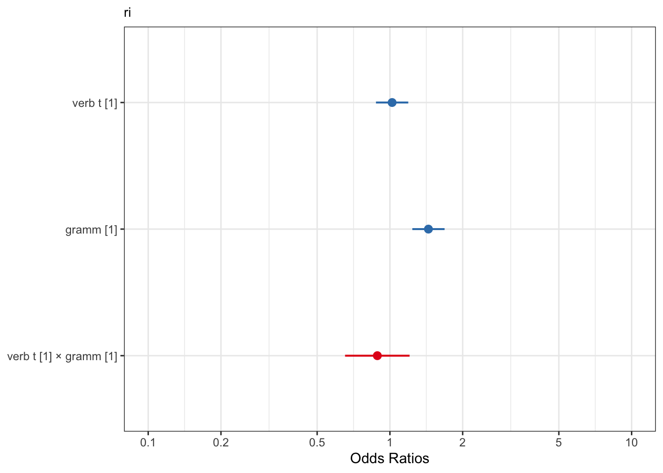

plot_model(fit_tense_ri, type = "eff",
           terms = "verb_t")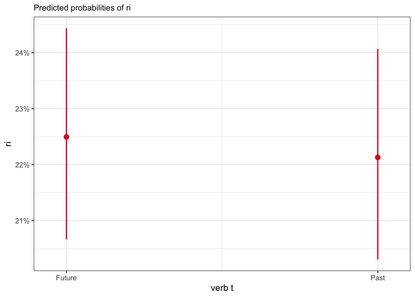

plot_model(fit_tense_ri, type = "eff",
           terms = "gramm")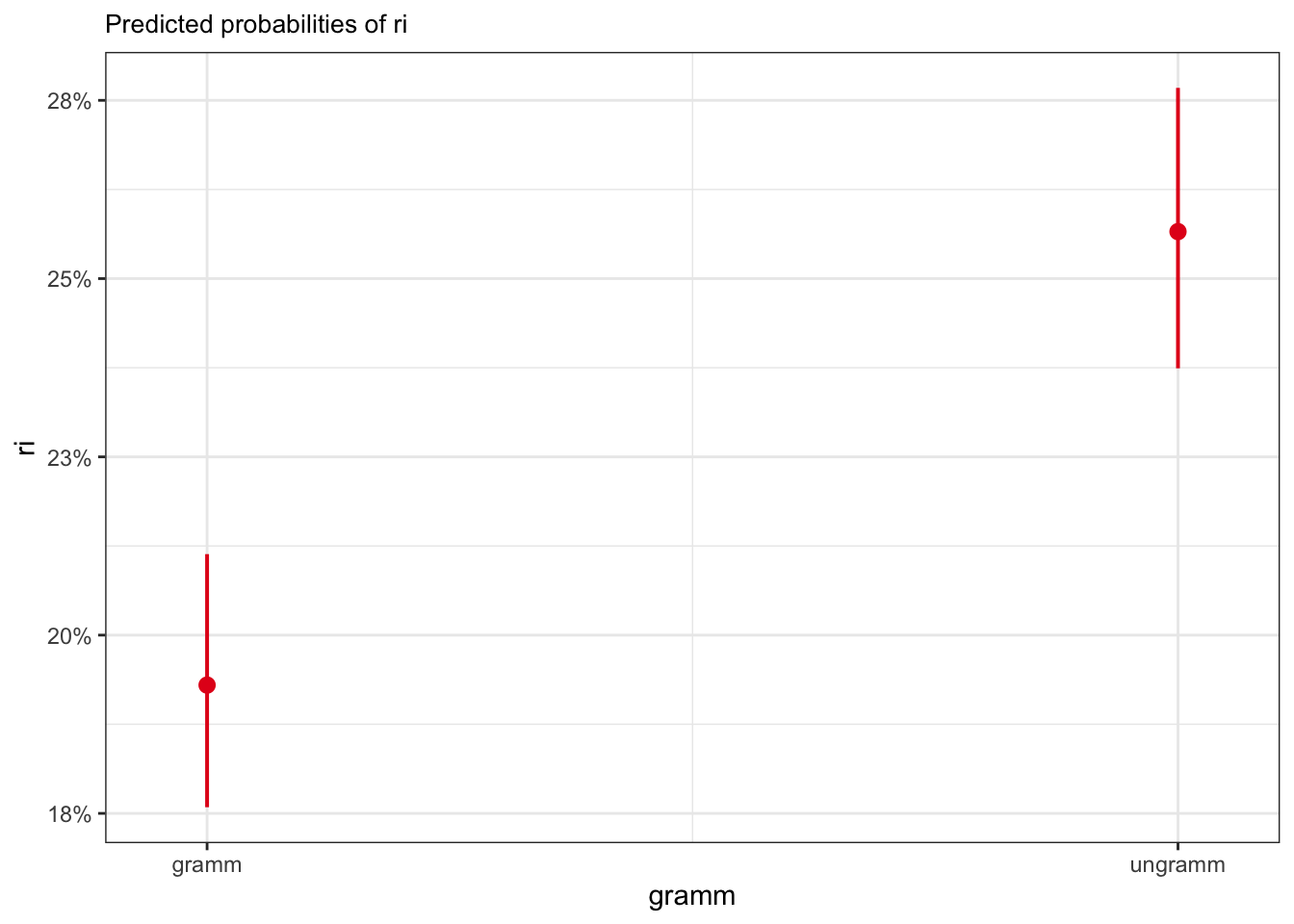

plot_model(fit_tense_ri, type = "int")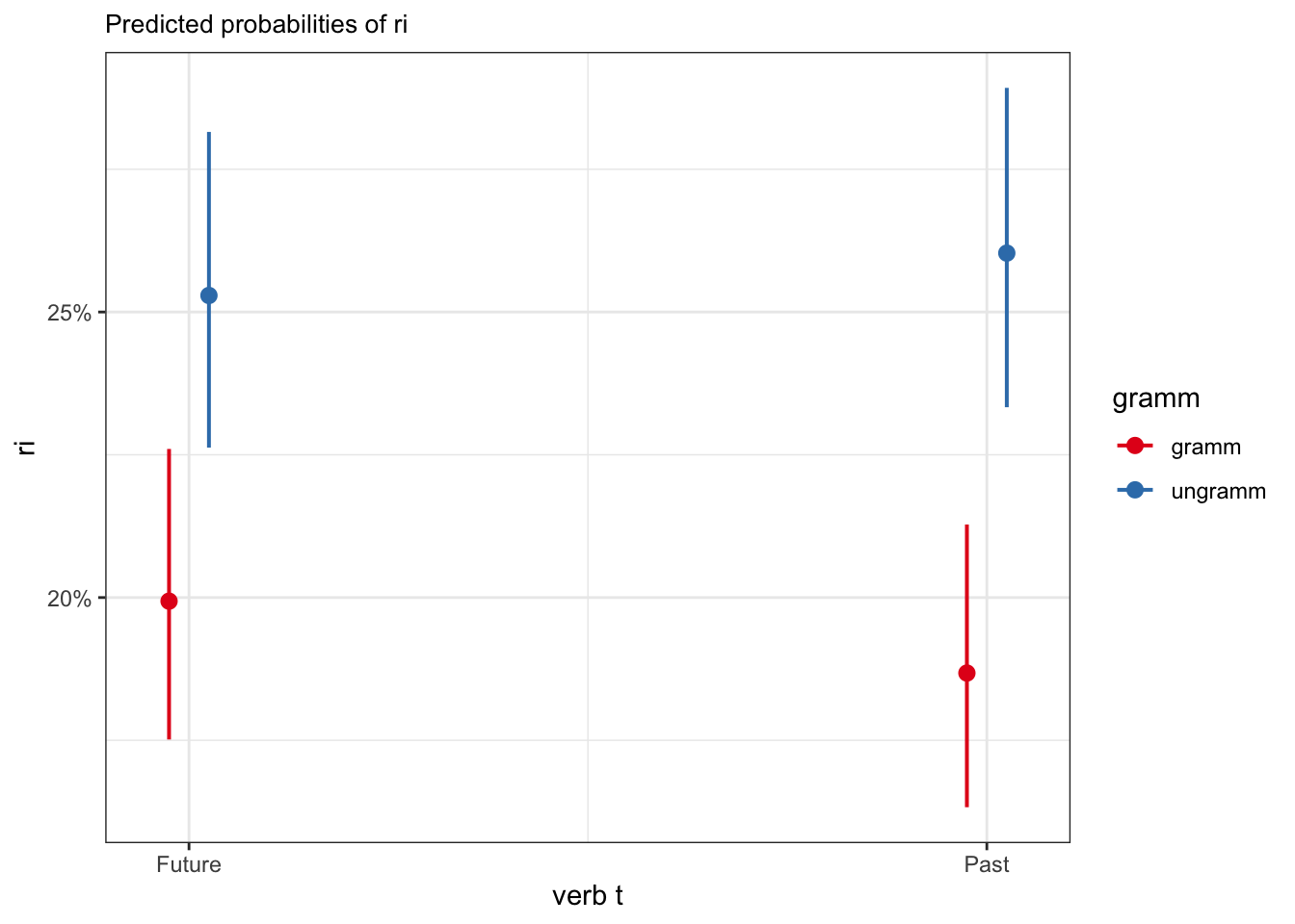

Or we can use the ggeffects package to extract summaries of effects, and then feed them into ggplot2.

library(ggeffects)

ggeffect(fit_tense_ri)

$verb_t
# Predicted probabilities of ri

verb_t | Predicted |     95% CI
-------------------------------
Future |      0.22 | 0.21, 0.24
Past   |      0.22 | 0.20, 0.24


$gramm
# Predicted probabilities of ri

gramm   | Predicted |     95% CI
--------------------------------
gramm   |      0.19 | 0.18, 0.21
ungramm |      0.26 | 0.24, 0.28


attr(,"class")
[1] "ggalleffects" "list"        
attr(,"model.name")
[1] "fit_tense_ri"

ggeffect(fit_tense_ri,
         terms = c("gramm", "verb_t"))

# Predicted probabilities of ri

verb_t: Future

gramm   | Predicted |     95% CI
--------------------------------
gramm   |      0.20 | 0.18, 0.23
ungramm |      0.25 | 0.23, 0.28

verb_t: Past

gramm   | Predicted |     95% CI
--------------------------------
gramm   |      0.19 | 0.16, 0.21
ungramm |      0.26 | 0.23, 0.29

6.5 Reporting

Sonderegger (2023) (Section 6.9) says the following:

Reporting a logistic regression model in a write-up is generally similar to reporting a linear regression model…Reporting a logistic regression model in a write-up is generally similar to reporting a linear regression model: the guidelines and rationale in section 4.6 for reporting individual coefficients and the whole model hold, with some adjustments.

We can produce such a table using the papaja package, as in Table 6.2.

library(papaja)

fit_tense_ri |> 
  apa_print() |>
  apa_table(caption = "Model summary for regressions in at the verb region. Estimates are given in log odds.")

Table 6.2: ?(caption)

(a) (#tab:tbl-glm-summary) Model summary for regressions in at the verb region. Estimates are given in log odds.

Predictor	\(b\)	95% CI	\(z\)	\(p\)
Intercept	-1.25	[-1.32, -1.17]	-31.81	< .001
Verb t1	0.02	[-0.13, 0.17]	0.27	.789
Gramm1	0.37	[0.21, 0.52]	4.68	< .001
Verb t1 \(\times\) Gramm1	-0.12	[-0.43, 0.19]	-0.76	.445

Or by extracting the model summary with tidy(), and even adding our probabilities, as in Table 6.3.

tidy(fit_tense_ri) |> 
  mutate(prob = plogis(estimate)) |> 
  relocate(prob, .after = std.error) |> 
  apa_table()

Table 6.3: ?(caption)

(a) (#tab:tbl-glm-summary2)

term	estimate	std.error	prob	statistic	p.value
(Intercept)	-1.25	0.04	0.22	-31.81	0.00
verb_t1	0.02	0.08	0.51	0.27	0.79
gramm1	0.37	0.08	0.59	4.68	0.00
verb_t1:gramm1	-0.12	0.16	0.47	-0.76	0.45

6.6 Summary

• we saw that the equation for a straight line boils down to its intercept and slope

• we fit our first linear model with a categorical predictor

Important terms

term	description/other terms
NA	NA
:----	:-----------------------

Important terms

Term	Definition	Equation/Code
Bernoulli distribution	NA	NA
plogis()	NA	NA
log odds	NA	NA

Learning Objectives

Today we learned…

• how to model binomial data with logistic regression
• how to interpret log-odds and odds ratio

Task

6.6.1 Regressions out

Using the same dataset, run a logistic model exploring regressions in (ri) at the adverb region (roi = "2"). Before you run the model, do you have any predictions? Try plotting the regressions in for this region first, and generate some summary tables to get an idea of the distributions of regressions in across conditions.

6.6.2 Dutch verb regularity

Load in the regularity data from the languageR package.

df_reg <-
  regularity |> 
  clean_names()

Regular and irregular Dutch verbs and selected lexical and distributional properties.

Our relevant variables will be:

• written_frequency: a numeric vector of logarithmically transformed frequencies in written Dutch (as available in the CELEX lexical database).
• regularity: a factor with levels irregular (1) and regular (0).
• verb: a factor with the verbs as levels.

1. Fit a logistic regression model to the data which predicts verb regularity by written frequency. Consider: What type of predictor variable do you have, and what steps should you take before fitting your model?

2. Print the model coefficients, e.g., using tidy().

3. Interpret the coefficients, either in log-odds or probabilities. Report your findings.

Session Info

Developed with Quarto using R version 4.4.0 (2024-04-24) (Puppy Cup) and RStudio version 2023.9.0.463 (Desert Sunflower), and the following packages:

sessionInfo()

R version 4.4.0 (2024-04-24)
Platform: aarch64-apple-darwin20
Running under: macOS Ventura 13.2.1

Matrix products: default
BLAS:   /Library/Frameworks/R.framework/Versions/4.4-arm64/Resources/lib/libRblas.0.dylib 
LAPACK: /Library/Frameworks/R.framework/Versions/4.4-arm64/Resources/lib/libRlapack.dylib;  LAPACK version 3.12.0

locale:
[1] en_US.UTF-8/en_US.UTF-8/en_US.UTF-8/C/en_US.UTF-8/en_US.UTF-8

time zone: Europe/Berlin
tzcode source: internal

attached base packages:
[1] stats     graphics  grDevices datasets  utils     methods   base     

other attached packages:
 [1] papaja_0.1.2        tinylabels_0.2.4    ggeffects_1.5.2    
 [4] sjPlot_2.8.15       gt_0.10.1           googlesheets4_1.1.1
 [7] kableExtra_1.4.0    knitr_1.43          patchwork_1.2.0    
[10] languageR_1.5.0     janitor_2.2.0       lme4_1.1-35.3      
[13] Matrix_1.7-0        broom_1.0.5         here_1.0.1         
[16] lubridate_1.9.3     forcats_1.0.0       stringr_1.5.1      
[19] dplyr_1.1.4         purrr_1.0.2         readr_2.1.5        
[22] tidyr_1.3.1         tibble_3.2.1        ggplot2_3.5.1      
[25] tidyverse_2.0.0     broman_0.80        

loaded via a namespace (and not attached):
 [1] DBI_1.2.2          rlang_1.1.3        magrittr_2.0.3     snakecase_0.11.1  
 [5] compiler_4.4.0     systemfonts_1.0.6  vctrs_0.6.5        pkgconfig_2.0.3   
 [9] crayon_1.5.2       fastmap_1.1.1      backports_1.4.1    labeling_0.4.3    
[13] effectsize_0.8.7   utf8_1.2.4         rmarkdown_2.24     tzdb_0.4.0        
[17] haven_2.5.4        nloptr_2.0.3       bit_4.0.5          xfun_0.40         
[21] jsonlite_1.8.7     highr_0.10         sjmisc_2.8.9       parallel_4.4.0    
[25] R6_2.5.1           RColorBrewer_1.1-3 stringi_1.8.3      boot_1.3-30       
[29] cellranger_1.1.0   estimability_1.5   Rcpp_1.0.12        modelr_0.1.11     
[33] parameters_0.21.6  pacman_0.5.1       nnet_7.3-19        splines_4.4.0     
[37] timechange_0.3.0   tidyselect_1.2.1   rstudioapi_0.16.0  effects_4.2-2     
[41] yaml_2.3.7         sjlabelled_1.2.0   curl_5.2.1         lattice_0.22-6    
[45] withr_3.0.0        bayestestR_0.13.2  coda_0.19-4.1      evaluate_0.21     
[49] survival_3.5-8     survey_4.4-2       xml2_1.3.6         pillar_1.9.0      
[53] carData_3.0-5      renv_1.0.7         insight_0.19.10    generics_0.1.3    
[57] vroom_1.6.5        rprojroot_2.0.4    hms_1.1.3          munsell_0.5.1     
[61] scales_1.3.0       minqa_1.2.6        xtable_1.8-4       glue_1.7.0        
[65] emmeans_1.10.1     tools_4.4.0        fs_1.6.3           mvtnorm_1.2-4     
[69] grid_4.4.0         mitools_2.4        datawizard_0.10.0  colorspace_2.1-0  
[73] nlme_3.1-164       performance_0.11.0 googledrive_2.1.1  cli_3.6.2         
[77] fansi_1.0.6        gargle_1.5.2       viridisLite_0.4.2  svglite_2.1.3     
[81] sjstats_0.18.2     gtable_0.3.5       sass_0.4.7         digest_0.6.33     
[85] htmlwidgets_1.6.4  farver_2.1.1       htmltools_0.5.8.1  lifecycle_1.0.4   
[89] httr_1.4.7         bit64_4.0.5        MASS_7.3-60.2     

References

Biondo, N., Soilemezidi, M., & Mancini, S. (2022). Yesterday is history, tomorrow is a mystery: An eye-tracking investigation of the processing of past and future time reference during sentence reading. Journal of Experimental Psychology: Learning, Memory, and Cognition, 48(7), 1001–1018. https://doi.org/10.1037/xlm0001053

Sonderegger, M. (2023). Regression Modeling for Linguistic Data.

Winter, B. (2019). Statistics for Linguists: An Introduction Using R. In Statistics for Linguists: An Introduction Using R. Routledge. https://doi.org/10.4324/9781315165547