setwd() depends on your entire machine’s folder structure
setwd() breaks when you
send your project folder to a collaborator
make your analyses open
change the location of your project folder
using slashes is also dependent on your operating system
The benefit of here()
uses the top-level directory of your project as the working directory
can separate folder names with a comma
here
Load the dataset using here
Install here (e.g., install.packages("here"))
Load here at the beginning of your package
or use here:: before calling a function
Use the here() function to load in your data
Inspect the dataset however you usually would (e.g., summary(), names(), etc.)
Save your script
here::here()
install package
In the Console
install.packages("here")
load package and call the here function
# load packagelibrary(here)# read in datadf_data <-read.csv(here("data", "data_lifetime_pilot.csv"))
or directly call the here function without loading the package
# read in data without loading heredf_data <-read.csv(here::here("data", "data_lifetime_pilot.csv"))
note that I stored the data with the prefix df_
df stands for dataframe
I recommend using object-type defining prefixes for all objects in your Environment
e.g., fit_ for models, fig_ for figures, sum_ for summaries, tbl_ for tables, etc.
Reproduce your analysis
Perform some data exploration (e.g., with names(), summary(), dplyr::glimpse(), whatever you typically do)
Save your script, then close RStudio/your Rproject.
Re-open the project. Can you re-run the script?
Learning objectives 🏁
Today we learned…
learn about project-oriented workflows ✅
create an RProject ✅
establish a self-contained project environment with here ✅
References
Bryan, J., & TAs, T. S. 545. (n.d.). R Basics and workflows. In STAT 545 Course materials. Retrieved May 6, 2024, from https://stat545.com/
Chromý, J., Brand, J., Laurinavichyute, A., & Lacina, R. (2023). Number agreement attraction in Czech and English comprehension: A direct experimental comparison. Glossa Psycholinguistics, 2(1), 1–20. https://doi.org/10.5070/G6011235
Wickham, H., Çetinkaya-Rundel, M., & Grolemund, G. (2023). R for Data Science (2nd ed.). https://r4ds.hadley.nz/
Wickham, H., & Grolemund, G. (2016). R for data science: Import, tidy, transform, visualize, and model data. " O’Reilly Media, Inc.".
Source Code
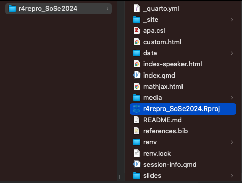
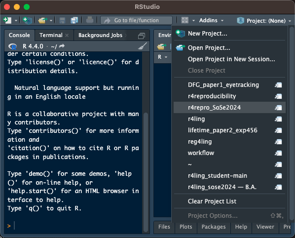
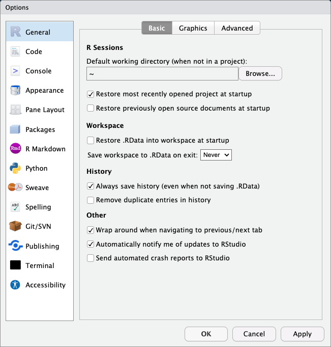
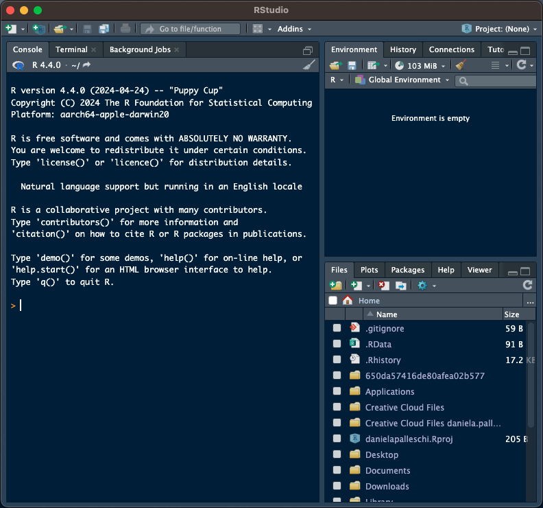
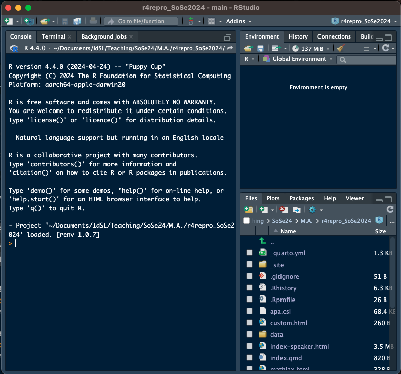
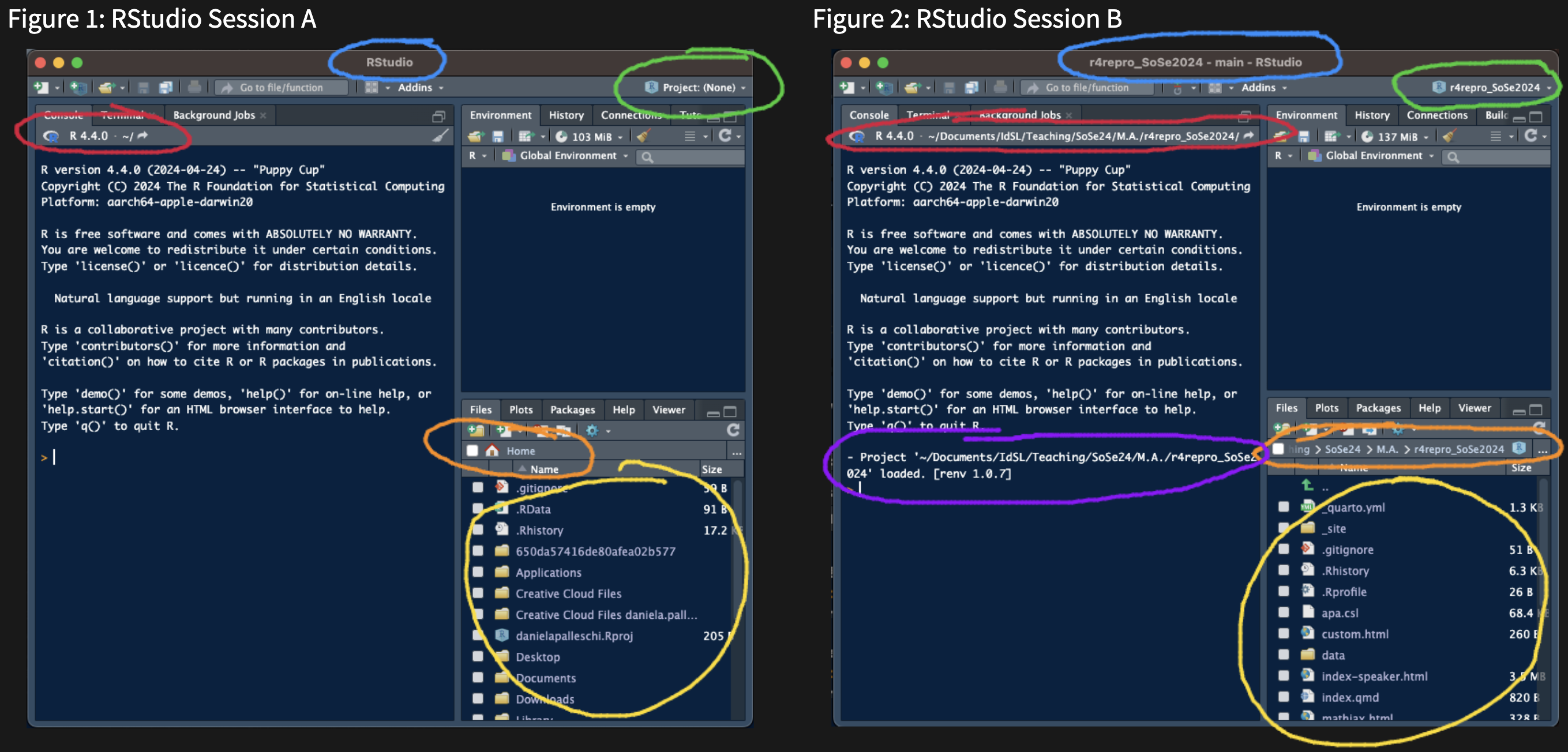
---title: "RProjects"subtitle: "Creating a project-oriented workflow in R"author: "Daniela Palleschi"institute: Humboldt-Universität zu Berlinlang: endate: 2024-08-22date-format: "ddd MMM D, YYYY"date-modified: last-modifiedlanguage: title-block-published: "Workshop Day 2" title-block-modified: "Last Modified"format: html: output-file: rprojects.html number-sections: false toc: true code-overflow: wrap code-tools: true embed-resources: false pdf: output-file: rprojects.pdf toc: true number-sections: false colorlinks: true code-overflow: wrap revealjs: footer: "SSOL 2024" output-file: rprojects_slides.html code-overflow: wrap theme: [dark] width: 1600 height: 900 # chalkboard: # src: chalkboard.json progress: true scrollable: true # smaller: true slide-number: c/t code-link: true incremental: true # number-sections: true toc: false toc-depth: 2 toc-title: 'Overview' navigation-mode: linear controls-layout: bottom-right fig-cap-location: top font-size: 0.6em slide-level: 4 embed-resources: false fig-align: center fig-dpi: 300editor_options: chunk_output_type: consolebibliography: references.bibcsl: ../../../apa.cslexecute: echo: false---```{r}#| echo: false#| eval: falserbbt::bbt_update_bib(here::here("slides", "day2", "rprojects", "rprojects.qmd"))```# Learning Objectives {.unnumbered .unlisted}Today we will...- learn about project-oriented workflows- create an RProject- use project-relative filepaths with the `here` package# Installation requirements- required installations/recent versions of: - R - version `4.4.0`, "Puppy Cup" - check current version with `R.version` - download/update: <https://cran.r-project.org/bin/macosx/> - RStudio - version `2023.12.1.402`, "Ocean Storm" - Help \> Check for updates - new install: <https://posit.co/download/rstudio-desktop/># Project-oriented workflow1. Folder structure: + keeping everything related to a project in one place + i.e., contained in a single folder, with subfolders as needed2. Project-relative working directory + the project folder should act as your working directory + all file paths should be relative to this folder## Folder structure- a core computer literacy skill + keep your Desktop as empty as possible + have a sensible folder structure + avoid mixing subfolders and files + i.e., if a folder contains subfolders, ideally it should not contain files# RProjects- in data analysis, using an IDE is beneficial + e.g., RStudio- most IDEs have their own implementation of a Project- in RStudio, this is the RProject + creates a `.Rproj` file in a project folder + stores project settings- you can have several RProjects open simultaneously + and run several scripts across projects simultaneously- most importantly, RProjects (can) centralise a specific project's workflow and file path- to read more about R Projects, check out [Section 6.2: Projects](https://r4ds.hadley.nz/workflow-scripts.html#projects) from @wickham_r_2023 [or [Ch. 8 - Workflow: Projects](https://r4ds.had.co.nz/workflow-projects.html) in @wickham_r_2016]## Creating a new Project- when? + whenever you're starting a new course or project which will use R- why? + to keep all the relavent materials in one place- where? + somewhere that makes sense, e.g., a folder called `SoSe2024` or `Mastersarbeit`- how? + `File > New Project > New Directory > New Project > [Directory name] > Create Project`### {.unnumbered .unlisted}::: {.callout-tip}# New RProjectCreate a new RProject for this workshop + `File > New Project > New Directory > New Project > [Directory name] > Create Project` + make sure you choose a sensible location:::## Opening a Project- to open a project, locate its `.Rproj` file and double-click- or if you're already in RStudio, you can use the `Project (None)` drop-down (top right):::: {.columns}::: {.column width="50%"}```{r}#| label: fig-click-open#| fig-cap: Double-click `.Rproj`#| out-width: "80%"knitr::include_graphics(here::here("media", "rstudio_click_open.png"))```:::::: {.column width="50%"}```{r}#| label: fig-project-open#| fig-cap: Open from RStudioknitr::include_graphics(here::here("media", "rstudio_project_open.png"))```:::::::## Adding a README file- `File > New File > Markdown File` (*not* R Markdown!) + add some text describing the purpose of this project + include your name, the date + use Markdown formatting (e.g., `#` for headings, `*italics*`, `**bold**`)- save as `README.md` in your project directory## Global RStudio options:::: {.columns}::: {.column width="50%"}```{r}#| label: fig-rstudio-settings#| fig-cap: RStudio settings for reproducibilityknitr::include_graphics(here::here("media", "RStudio_global-options.png"))```:::::: {.column width="50%"}- `Tools > Global Options` + **Workspace**: Restore .RData into workspace at startup: NO + Save workspace to .RData on exit: Never- this will ensure that you are always starting with a clean slate + and that your code is not dependent on some pacakge or object you created in another session- this is also how RMarkdown and Quarto scripts run + they start with an empty environment and run the script linearly:::::::## {.unnumbered .unlisted}::: {.callout-tip}## Global settingsChange your Global Options so that + **Workspace**: Restore .RData into workspace at startup: NO + Save workspace to .RData on exit: Never:::## Identifying your RProject- there are a ways to check which (if any) RProject you're in + there are 6 differences between xyzfig-noproject and xyzfig-project + which is in an RProject session?::: {.panel-tabset}### Spot the differences:::: {.columns}::: {.column width="45%"}```{r}#| label: fig-noproject#| fig-cap: RStudio Session Aknitr::include_graphics(here::here("media", "rstudio_noproject.png"))```:::::: {.column width="5%"}:::::: {.column width="45%"}```{r}#| label: fig-project#| fig-cap: RStudio Session Bknitr::include_graphics(here::here("media", "rstudio_project.png"))```:::::::### Show the differences```{r}knitr::include_graphics(here::here("media", "rproject_spot-the-diffs.png"))```:::# Folder structure- some folders you'll typically want to have: + `data`: containing your dataset(s) + `scripts` (or `analyses`, etc.): containing any analysis scripts + `manuscript`: containing any write-ups of your results + `materials`: containing relevant experiment materials (e.g., stimuli)- let's just create the first 2 (`data` and `scripts`)### `data/`- do you have "raw", i.e., pre-processed data? + if so, you might want to create a `raw` sub-folder + and any other relevant sub-folders (e.g., `processed` or `tidy`)- download [the dataset](https://osf.io/ushpw) from the workshop repo [from @chromy_number_2023] + *or*, move a dataset of your own to this folder### `scripts/`- try to create a single script for each "product" + e.g., anonymised data, 'cleaned' data, data exploration, visualisation, analyses, etc.- you can create sub-folders as the project develops and move scripts around + for now, let's create a new script to take a look at our data### {.unnumbered .unlisted}::: {.callout-tip}## New scriptCreate a new Quarto script:1. `File > New File > Quarto Document`3. Add a title2. Uncheck the `Use Visual Editor` box4. Click `Create`5. Save it in your `scripts/` folder: `File > Save as...`:::### Load in the data- load in the data however you normally would + e.g., `readr::read_csv()`# `here`-package- `here` package [@here-package] enables file referencing + avoids the use of `setwd()````{r}#| label: fig-here#| fig-cap: Illustration by [Allison Horst](https://github.com/allisonhorst)knitr::include_graphics(here::here("media", "Horst_here.png"))```## The problem with `setwd()`> If the first line of your R script is>> `setwd("C:\Users\jenny\path\that\only\I\have")`>> I will come into your office and SET YOUR COMPUTER ON FIRE🔥.--- [Jenny Bryan](https://x.com/hadleywickham/status/940021008764846080)- `setwd()` depends on your entire machine's folder structure- `setwd()` breaks when you + send your project folder to a collaborator + make your analyses open + change the location of your project folder- using slashes is also dependent on your operating system## The benefit of `here()`- uses the top-level directory of your project as the working directory- can separate folder names with a comma## {.unlisted .unnumbered}::: {.callout-tip}# `here`Load the dataset using `here`1. Install `here` (e.g., `install.packages("here")`)2. Load `here` at the beginning of your package + or use `here::` before calling a function3. Use the `here()` function to load in your data4. Inspect the dataset however you usually would (e.g., `summary()`, `names()`, etc.)4. Save your script:::## `here::here()`- install package```{r filename = "In the Console"}#| eval: false#| echo: trueinstall.packages("here")```- load package and call the `here` function```{r}#| eval: false#| echo: true# load packagelibrary(here)# read in datadf_data <-read.csv(here("data", "data_lifetime_pilot.csv"))```- or directly call the `here` function without loading the package```{r}#| eval: false#| echo: true# read in data without loading heredf_data <-read.csv(here::here("data", "data_lifetime_pilot.csv"))```- note that I stored the data with the prefix `df_` + `df` stands for dataframe- I recommend using object-type defining prefixes for all objects in your Environment + e.g., `fit_` for models, `fig_` for figures, `sum_` for summaries, `tbl_` for tables, etc.## {.unlisted .unnumbered}::: {.callout-tip}# Reproduce your analysis1. Perform some data exploration (e.g., with `names()`, `summary()`, `dplyr::glimpse()`, whatever you typically do)1. Save your script, then close RStudio/your Rproject.2. Re-open the project. Can you re-run the script?:::# Learning objectives 🏁 {.unnumbered .unlisted .uncounted}Today we learned...- learn about project-oriented workflows ✅- create an RProject ✅- establish a self-contained project environment with `here` ✅# References {.unlisted .unnumbered visibility="uncounted"}---nocite: | @bryan_what_nodate-1 @bryan_chapter_nodate @noauthor_using_2024---::: {#refs custom-style="Bibliography"}:::